
多任务学习中损失函数权重的自动调整
多任务学习;同方差不确定性;辅助任务;损失函数权重调参;
0 引言
多任务学习:给定 m m m 个学习任务,其中所有或一部分任务是相关但并不完全一样的,多任务学习的目标是通过使用这 m m m 个任务中包含的知识来帮助提升各个任务的性能。
多任务学习有多种实现的范式,但通常我们认为:一个模型包含多个目标函数同时进行训练,完成多个任务,这是广义上的多任务学习。下图描述了一个典型的多任务学习场景,模型同时完成语义分割、实例分割和深度估计任务。

L t o t a l = ∑ i w i L i L_{total} = \sum_{i}^{} w_iL_i Ltotal=i∑wiLi
多任务学习中,模型的训练通常由多个损失函数加权得到损失,其中不同任务所使用的损失函数的纲量,以及该任务的重要程度是需要人为设参的,这使得我们可能会花费大量时间去调参,或是使用业界统一的参数(但这是否是最优的有待商榷)。所以,考虑能否使用自动调整各损失函数的权重,以解放训练效率甚至是优化模型的性能。
从这里也引出思考:能否将这项工作应用于单任务多输出模型(例如OCRNet、BiSeNetV2、U 2 ^2 2Net)或是单任务混合损失的权重调参上(例如语义分割中CELoss+LovaszSoftmaxLoss通常是0.8+0.2)。
下面由代码引入。
1 数据集定义
以下数据集定义了两个任务回归任务,我们将使用同一个特征 x x x 完成两个线性回归 y 1 y_1 y1 和 y 2 y_2 y2 任务,这两个任务的标签具有不同的斜率、截距以及方差(可自行修改)。
import matplotlib.pyplot as plt
%matplotlib inline
import paddle
import numpy as np
class RegressionDataset(paddle.io.Dataset):
    def __init__(self, sample_nums):
        super(RegressionDataset, self).__init__()

        assert isinstance(sample_nums, int) and sample_nums > 0
        self.sample_nums = sample_nums
        self.x = np.random.randn(self.sample_nums, 1)
        self.y1 = self.generate_targets(w=-2, b=1, sigma=3.0)
        self.y2 = self.generate_targets(w=1.5, b=3, sigma=0.5)

    def __getitem__(self, idx):
        return (np.float32(self.x[idx]),
                np.float32(self.y1[idx]),
                np.float32(self.y2[idx]))

    def __len__(self):
        return self.sample_nums

    def generate_targets(self, w, b, sigma):
        return self.x * w + b + sigma * np.random.randn(self.sample_nums, 1)
np.random.seed(1024)
dataset = RegressionDataset(sample_nums=300)
plt.figure(figsize=(6, 4))
plt.scatter(dataset.x, dataset.y1)
plt.scatter(dataset.x, dataset.y2)
plt.legend([r'y1($\sigma=3$)', r'y2($\sigma=0.5$)'], loc=0)
plt.show()
![[外链图片转存失败,源站可能有防盗链机制,建议将图片保存下来直接上传(img-z2gSYdno-1643451871589)(output_5_0.png)]](https://i-blog.csdnimg.cn/blog_migrate/09c3c7fc240a5e95ae09c58b91c8682a.png)
2 模型定义
此处定义一个简单的回归任务模型,但并不采用权重共享(可自行修改)。
class MTLRegressionModel(paddle.nn.Layer):
    def __init__(self, in_nums, hidden_nums, out_nums):
        super(MTLRegressionModel, self).__init__()

        assert isinstance(in_nums, int) and in_nums > 0
        assert isinstance(hidden_nums, int) and hidden_nums > 0
        assert isinstance(out_nums, int) and out_nums > 0
        self.net1 = paddle.nn.Sequential(
            paddle.nn.Linear(in_features=in_nums, out_features=hidden_nums),
            paddle.nn.ReLU(),
            paddle.nn.Linear(in_features=hidden_nums, out_features=out_nums))
        self.net2 = paddle.nn.Sequential(
            paddle.nn.Linear(in_features=in_nums, out_features=hidden_nums),
            paddle.nn.ReLU(),
            paddle.nn.Linear(in_features=hidden_nums, out_features=out_nums))

    def forward(self, inputs):
        return [self.net1(inputs), self.net2(inputs)]
model = MTLRegressionModel(in_nums=1, hidden_nums=512, out_nums=1)
batch_size = 16
paddle.summary(model, input_size=(batch_size, 1))
对于以上模型,通常会选择两个均方误差函数MSELoss,加权为 1 : 1 1:1 1:1 进行训练,但这个加权方案对于模型训练是最优的吗?
3 同方差不确定性
(Alex Kendall等人,2018) 提出,使用同方差不确定性调整权重系数,取得了较好效果。
通常深度模型建模中存在两种不确定性,分别是认知不确定性(欠拟合等)和偶然不确定性(数据信息限制等),其中偶然不确定性又可以划分为同方差不确定性(数据依赖)和异方差不确定性(任务依赖)。如引言中所展示的图片,多任务学习通常是同一个数据集的不同任务,所以考虑同方差不确定性来衡量损失函数的权重。
下面从回归和分类的角度分别推导了基于同方差不确定性的损失函数。
3.1 回归损失
输出建模(具有观测噪声):
p ( y ∣ f W ( x ) ) = N ( f W ( x ) , σ 2 ) p(y|f^W(x)) = \mathcal{N}(f^W(x),\sigma^2) p(y∣fW(x))=N(fW(x),σ2)
最大化概率模型的对数似然:
log p ( y ∣ f W ( x ) ) = log N ( f W ( x ) , σ 2 ) = log ( 1 2 π σ e − ∣ ∣ y − f W ( x ) ∣ ∣ 2 2 σ 2 ) ∝ − 1 2 σ 2 ∣ ∣ y − f W ( x ) ∣ ∣ 2 − log σ \log p(y|f^W(x)) = \log \mathcal{N}(f^W(x),\sigma^2) \\ = \log (\frac{1}{\sqrt{2\pi}\sigma} e^{-\frac{||y-f^W(x)||^2}{2\sigma^2}} ) \\ ∝ -\frac{1}{2\sigma^2}||y-f^W(x)||^2-\log \sigma logp(y∣fW(x))=logN(fW(x),σ2)=log(2πσ1e−2σ2∣∣y−fW(x)∣∣2)∝−2σ21∣∣y−fW(x)∣∣2−logσ
假设同时进行两个回归任务,有如下输出建模:
p ( y 1 , y 2 ∣ f W ( x ) ) = p ( y 1 ∣ f W ( x ) ) ⋅ p ( y 2 ∣ f W ( x ) ) = N ( y 1 ; f W ( x ) , σ 1 2 ) ⋅ N ( y 2 ; f W ( x ) , σ 2 2 ) p(y_1,y_2|f^W(x)) = p(y_1|f^W(x))\cdot p(y_2|f^W(x)) \\ = \mathcal{N}(y_1;f^W(x),\sigma_1^2) \cdot \mathcal{N}(y_2;f^W(x),\sigma_2^2) p(y1,y2∣fW(x))=p(y1∣fW(x))⋅p(y2∣fW(x))=N(y1;fW(x),σ12)⋅N(y2;fW(x),σ22)
最大化以上对数似然,等价于最小化如下目标函数:
L ( W , σ 1 , σ 2 ) = − log ( p ( y 1 , y 2 ∣ f W ( x ) ) ) ∝ 1 2 σ 1 2 ∣ ∣ y − f W ( x ) ∣ ∣ 2 + log σ 1 + 1 2 σ 2 2 ∣ ∣ y − f W ( x ) ∣ ∣ 2 + log σ 2 = 1 2 σ 1 2 L 1 ( W ) + log σ 1 + 1 2 σ 2 2 L 2 ( W ) + log σ 2 \mathcal{L}(W,\sigma_1,\sigma_2) = -\log(p(y_1,y_2|f^W(x))) \\ ∝ \frac{1}{2\sigma_1^2}||y-f^W(x)||^2+\log \sigma_1+\frac{1}{2\sigma_2^2}||y-f^W(x)||^2+\log \sigma_2 \\= \frac{1}{2\sigma_1^2}\mathcal{L}_1(W) +\log \sigma_1+\frac{1}{2\sigma_2^2}\mathcal{L}_2(W) +\log \sigma_2 L(W,σ1,σ2)=−log(p(y1,y2∣fW(x)))∝2σ121∣∣y−fW(x)∣∣2+logσ1+2σ221∣∣y−fW(x)∣∣2+logσ2=2σ121L1(W)+logσ1+2σ221L2(W)+logσ2
噪声 σ \sigma σ 表示同方差不确定性大小,而末尾的 l o g σ log \sigma logσ 相当于正则项。
3.2 分类损失
输出建模(引入温度系数 σ \sigma σ,吉布斯分布):
p ( y ∣ f W ( x ) ) = softmax ( 1 σ 2 f W ( x ) ) ) p(y|f^W(x)) = \text{softmax}(\frac{1}{\sigma^2}f^W(x))) p(y∣fW(x))=softmax(σ21fW(x)))
分类模型的对数似然:
log p ( y ∣ f W ( x ) ) = log softmax ( 1 σ 2 f W ( x ) ) ) = log exp ( 1 σ 2 f c W ( x ) ) ∑ c exp ( 1 σ 2 f c W ( x ) ) = 1 σ 2 f c W ( x ) − log ∑ c exp ( 1 σ 2 f c W ( x ) ) = 1 σ 2 ( f c W ( x ) − log ∑ c exp ( f c W ( x ) ) ) + 1 σ 2 log ∑ c exp ( f c W ( x ) ) − log ∑ c exp ( 1 σ 2 f c W ( x ) ) = 1 σ 2 ( log exp ( f c W ( x ) ) ∑ c exp ( f c W ( x ) ) ) + log ( ∑ c exp ( f c W ( x ) ) ) 1 σ 2 − log ∑ c exp ( 1 σ 2 f c W ( x ) ) = 1 σ 2 ( log exp ( f c W ( x ) ) ∑ c exp ( f c W ( x ) ) ) + log ( ∑ c exp ( f c W ( x ) ) ) 1 σ 2 − log ∑ c exp ( 1 σ 2 f c W ( x ) ) = 1 σ 2 ( log softmax ( f W ( x ) ) ) + log ( ∑ c exp ( f c W ( x ) ) ) 1 σ 2 ∑ c exp ( 1 σ 2 f c W ( x ) ) \log p(y|f^W(x)) = \log \text{softmax}(\frac{1}{\sigma^2}f^W(x))) \\ = \log \frac{\exp(\frac{1}{\sigma^2}f_c^W(x))}{\sum_{c}^{}\exp(\frac{1}{\sigma^2}f_c^W(x))} \\ = \frac{1}{\sigma^2}f_c^W(x)-\log \sum_{c}^{}\exp(\frac{1}{\sigma^2}f_c^W(x)) \\ = \frac{1}{\sigma^2}(f_c^W(x)-\log \sum_{c}^{}\exp(f_c^W(x))) + \frac{1}{\sigma^2}\log \sum_{c}^{}\exp(f_c^W(x))-\log \sum_{c}^{}\exp(\frac{1}{\sigma^2}f_c^W(x)) \\ = \frac{1}{\sigma^2}(\log \frac{\exp(f_c^W(x))}{\sum_{c}^{}\exp(f_c^W(x))}) + \log (\sum_{c}^{}\exp(f_c^W(x)))^{\frac{1}{\sigma^2}}-\log \sum_{c}^{}\exp(\frac{1}{\sigma^2}f_c^W(x)) \\ = \frac{1}{\sigma^2}(\log \frac{\exp(f_c^W(x))}{\sum_{c}^{}\exp(f_c^W(x))}) + \log (\sum_{c}^{}\exp(f_c^W(x)))^{\frac{1}{\sigma^2}}-\log \sum_{c}^{}\exp(\frac{1}{\sigma^2}f_c^W(x)) \\ = \frac{1}{\sigma^2}(\log \text{softmax}(f^W(x))) + \log \frac{(\sum_{c}^{}\exp(f_c^W(x)))^{\frac{1}{\sigma^2}}}{ \sum_{c}^{}\exp(\frac{1}{\sigma^2}f_c^W(x))} logp(y∣fW(x))=logsoftmax(σ21fW(x)))=log∑cexp(σ21fcW(x))exp(σ21fcW(x))=σ21fcW(x)−logc∑exp(σ21fcW(x))=σ21(fcW(x)−logc∑exp(fcW(x)))+σ21logc∑exp(fcW(x))−logc∑exp(σ21fcW(x))=σ21(log∑cexp(fcW(x))exp(fcW(x)))+log(c∑exp(fcW(x)))σ21−logc∑exp(σ21fcW(x))=σ21(log∑cexp(fcW(x))exp(fcW(x)))+log(c∑exp(fcW(x)))σ21−logc∑exp(σ21fcW(x))=σ21(logsoftmax(fW(x)))+log∑cexp(σ21fcW(x))(∑cexp(fcW(x)))σ21
假设同时进行回归和分类任务,有如下目标函数:
L ( W , σ 1 , σ 2 ) = − log ( p ( y 1 , y 2 = c ∣ f W ( x ) ) ) = − log N ( y 1 ; f W ( x ) , σ 1 2 ) ⋅ softmax ( y 2 = c ; f W ( x ) , σ 2 2 ) = 1 2 σ 1 2 ∣ ∣ y − f W ( x ) ∣ ∣ 2 + log σ 1 − log p ( y 2 = c ; f W ( x ) , σ 2 2 ) = 1 2 σ 1 2 ∣ ∣ y − f W ( x ) ∣ ∣ 2 + log σ 1 − 1 σ 2 2 ( log softmax ( f W ( x ) ) ) − log ( ∑ c exp ( f c W ( x ) ) ) 1 σ 2 2 ∑ c exp ( 1 σ 2 2 f c W ( x ) ) = 1 2 σ 1 2 ∣ ∣ y − f W ( x ) ∣ ∣ 2 + log σ 1 + 1 σ 2 2 ( − log softmax ( f W ( x ) ) ) + log ∑ c exp ( 1 σ 2 2 f c W ( x ) ) ( ∑ c exp ( f c W ( x ) ) ) 1 σ 2 2 \mathcal{L}(W,\sigma_1,\sigma_2) = -\log(p(y_1,y_2=c|f^W(x))) \\ = -\log \mathcal{N}(y_1;f^W(x),\sigma_1^2)\cdot \text{softmax}(y_2=c;f^W(x),\sigma_2^2) \\ = \frac{1}{2\sigma_1^2}||y-f^W(x)||^2+\log \sigma_1-\log p(y_2=c;f^W(x),\sigma_2^2) \\ = \frac{1}{2\sigma_1^2}||y-f^W(x)||^2+\log \sigma_1 - \frac{1}{\sigma_2^2}(\log \text{softmax}(f^W(x))) - \log \frac{(\sum_{c}^{}\exp(f_c^W(x)))^{\frac{1}{\sigma_2^2}}}{ \sum_{c}^{}\exp(\frac{1}{\sigma_2^2}f_c^W(x))} \\ = \frac{1}{2\sigma_1^2}||y-f^W(x)||^2+\log \sigma_1 + \frac{1}{\sigma_2^2}(-\log \text{softmax}(f^W(x))) + \log \frac{ \sum_{c}^{}\exp(\frac{1}{\sigma_2^2}f_c^W(x))}{(\sum_{c}^{}\exp(f_c^W(x)))^{\frac{1}{\sigma_2^2}}} L(W,σ1,σ2)=−log(p(y1,y2=c∣fW(x)))=−logN(y1;fW(x),σ12)⋅softmax(y2=c;fW(x),σ22)=2σ121∣∣y−fW(x)∣∣2+logσ1−logp(y2=c;fW(x),σ22)=2σ121∣∣y−fW(x)∣∣2+logσ1−σ221(logsoftmax(fW(x)))−log∑cexp(σ221fcW(x))(∑cexp(fcW(x)))σ221=2σ121∣∣y−fW(x)∣∣2+logσ1+σ221(−logsoftmax(fW(x)))+log(∑cexp(fcW(x)))σ221∑cexp(σ221fcW(x))
化简:定义回归损失为 L 1 ( W ) = ∥ y − f W ( x ) ∥ 2 \mathcal{L}_1(W)=\|y-f^W(x)\|^2 L1(W)=∥y−fW(x)∥2,分类损失为 L 2 ( W ) = − log softmax ( f W ( x ) ) \mathcal{L}_2(W)=-\log \text{softmax}(f^W(x)) L2(W)=−logsoftmax(fW(x)),作近似 1 σ 2 ∑ c exp ( 1 σ 2 2 f c W ( x ) ) ≈ ( ∑ c exp ( f c W ( x ) ) ) 1 σ 2 2 \frac{1}{\sigma_2}\sum_{c}^{}\exp(\frac{1}{\sigma_2^2}f_c^W(x))≈(\sum_{c}^{}\exp(f_c^W(x)))^{\frac{1}{\sigma_2^2}} σ21∑cexp(σ221fcW(x))≈(∑cexp(fcW(x)))σ221,以上目标函数的近似结果为:
L ( W , σ 1 , σ 2 ) = 1 2 σ 1 2 L 1 ( W ) + log σ 1 + 1 σ 2 2 L 2 ( W ) + log σ 2 \mathcal{L}(W,\sigma_1,\sigma_2) = \frac{1}{2\sigma_1^2}\mathcal{L}_1(W)+\log \sigma_1+\frac{1}{\sigma_2^2}\mathcal{L}_2(W)+\log \sigma_2 L(W,σ1,σ2)=2σ121L1(W)+logσ1+σ221L2(W)+logσ2
3.3 结论
引入观测噪声 σ k \sigma_k σk,有如下损失函数:
L ( W , σ 1 , . . . , σ K ) = ∑ k = 1 K 1 2 σ k 2 L k ( W ) + log σ k \mathcal{L}(W,\sigma_1,...,\sigma_K) = \sum_{k=1}^{K}\frac{1}{2\sigma_k^2}\mathcal{L}_k(W)+\log \sigma_k L(W,σ1,...,σK)=k=1∑K2σk21Lk(W)+logσk
训练时,定义 log σ 2 \log \sigma^2 logσ2 为可训练变量,可以限制变化范围,规避分母为0异常。
class MTLLoss(paddle.nn.Layer):
    def __init__(self, task_nums):
        super(MTLLoss, self).__init__()
        x = paddle.zeros([task_nums], dtype='float32')
        self.log_var2s = paddle.create_parameter(
            shape=x.shape,
            dtype=str(x.numpy().dtype),
            default_initializer=paddle.nn.initializer.Assign(x))

    def forward(self, logit_list, label_list):
        loss = 0
        for i in range(len(self.log_var2s)):
            mse = (logit_list[i] - label_list[i]) ** 2
            pre = paddle.exp(-self.log_var2s[i])
            loss += paddle.sum(pre * mse + self.log_var2s[i], axis=-1)
        return paddle.mean(loss)
mtl_loss = MTLLoss(task_nums=2)
paddle.summary(mtl_loss, input_size=[(batch_size, 1), (batch_size, 1)])
4 训练参数与训练
此处需要注意,优化器也要载入损失函数模型的参数。
dataloader = paddle.io.DataLoader(
    dataset,
    batch_size=batch_size,
    shuffle=True)

parameters = model.parameters()
parameters.append(*mtl_loss.parameters())
optimizer = paddle.optimizer.Adam(
    learning_rate=0.0003,
    parameters=parameters)
开始训练,尝试1500个轮次,并保存每轮的损失和两个可训练参数。
loss_list, param_list = [], []
for epoch in range(1, 1501):
    model.train()
    loss_per_epoch = 0
    for x, y1, y2 in dataloader:
        logit_list = model(x)
        loss = mtl_loss(logit_list, [y1, y2])

        loss.backward()
        optimizer.step()
        optimizer.clear_grad()

        loss_per_epoch += loss.numpy()[0]

    loss_list.append(loss_per_epoch / len(dataset))
    param_list.append(mtl_loss.log_var2s.numpy())
5 训练结果
下面绘制<损失变化曲线图>和<同方差参数变化曲线图>。
plt.figure(figsize=(6, 8))
plt.subplot(211)
plt.title('train loss')
plt.plot(loss_list)

plt.subplot(212)
sigma_list = np.sqrt(np.exp(param_list))
plt.title(r'$\sigma_k$: ' + f'{sigma_list[-1]}')
plt.plot(sigma_list[:, 0])
plt.plot(sigma_list[:, 1])
plt.legend([r'$\sigma_1$', r'$\sigma_2$'])

plt.tight_layout()
plt.show()
![[外链图片转存失败,源站可能有防盗链机制,建议将图片保存下来直接上传(img-zlATET1a-1643451871590)(output_23_0.png)]](https://i-blog.csdnimg.cn/blog_migrate/76a641118c86758f76958aeaf2c09724.png)
以上可以观察到,训练约在800轮次趋于收敛。
在训练集上重新预测,得到拟合的散点。
pred_list = []
for x, y1, y2 in dataset:
    x = paddle.to_tensor(x, dtype='float32')
    x = paddle.expand(x, shape=(1, 1))
    logit_list = model(x)
    logit_list = [paddle.squeeze(item).numpy() for item in logit_list]
    pred_list.append(logit_list)
pred_list = np.array(pred_list)
plt.figure(figsize=(6, 6))
plt.scatter(dataset.x, dataset.y1)
plt.scatter(dataset.x, dataset.y2)
plt.scatter(dataset.x, pred_list[:, 0])
plt.scatter(dataset.x, pred_list[:, 1])
plt.legend(
    [r'y1($\sigma=3$)',
     r'y2($\sigma=0.5$)',
     'pred_y1(σ=%0.4f)' % sigma_list[-1][0],
     'pred_y2(σ=%.4f)' % sigma_list[-1][1]],
    loc=0)
plt.show()
![[外链图片转存失败,源站可能有防盗链机制,建议将图片保存下来直接上传(img-i4RYIL0b-1643451871590)(output_26_0.png)]](https://i-blog.csdnimg.cn/blog_migrate/c311f0db15e24f2469df50bfd5fa6676.png)
值得一提的是:可训练参数( p r e d _ y ∗ pred\_y* pred_y∗)和我们设定的高斯分布方差( y ∗ y* y∗)非常接近,如果增加训练样本可能会更加逼近,不妨自行实验。
6 PaddleSeg混合损失
(Lukas Liebel等人,2018)指出,辅助任务可以优化训练速度和网络性能,并对以上方法改进,以防止训练损失变为负数(其实这和我们选择 l o g σ 2 log\ \sigma ^2 log σ2 作为训练参数类似,这里在正则化项中加了1):
L c o m b ( x , y T , y T ′ ; ω T ) = ∑ τ ∈ T L τ ( x , y τ , y τ ′ ; ω τ ) ⋅ c τ \mathrm{L}_{\mathrm{comb}}\left(x, y_{\mathcal{T}}, y_{\mathcal{T}}^{\prime} ; \omega_{\mathcal{T}}\right)=\sum_{\tau \in \mathcal{T}} \mathrm{L}_{\tau}\left(x, y_{\tau}, y_{\tau}^{\prime} ; \omega_{\tau}\right) \cdot c_{\tau} Lcomb(x,yT,yT′;ωT)=τ∈T∑Lτ(x,yτ,yτ′;ωτ)⋅cτ
L T ( x , y T , y T ′ ; ω T ) = ∑ τ ∈ T 1 2 ⋅ c τ 2 ⋅ L τ ( x , y τ , y τ ′ ; ω τ ) + ln ( 1 + c τ 2 ) \begin{aligned} \mathrm{L}_{\mathcal{T}}\left(x, y_{\mathcal{T}}, y_{\mathcal{T}}^{\prime} ; \omega_{\mathcal{T}}\right)=& \sum_{\tau \in \mathcal{T}} \frac{1}{2 \cdot c_{\tau}^{2}} \cdot \mathrm{L}_{\tau}\left(x, y_{\tau}, y_{\tau}^{\prime} ; \omega_{\tau}\right) +\ln \left(1+c_{\tau}^{2}\right) \end{aligned} LT(x,yT,yT′;ωT)=τ∈T∑2⋅cτ21⋅Lτ(x,yτ,yτ′;ωτ)+ln(1+cτ2)
尝试将该方法应用于混合损失函数权重的调参,下面 PaddleSeg 为例编写损失函数,初始化优化器也要注意载入该损失函数的参数。以下代码组运行了两次得到对比结果,分别为自权重损失和固定权重,自己运行时注意保存路径。
!pip install paddleseg==2.4.0
import numpy as np
import random
import paddle
import paddleseg
import paddleseg.transforms as T

from paddleseg.cvlibs import manager
from paddleseg.datasets import OpticDiscSeg
from paddleseg.models import MixedLoss, CrossEntropyLoss, DiceLoss
random.seed(1024)
paddle.seed(1024)
np.random.seed(1024)
transforms = [T.Resize(target_size=(512, 512)), T.Normalize()]

train_dataset = OpticDiscSeg(
    dataset_root='data/optic_disc_seg',
    transforms=transforms,
    mode='train')
val_dataset = OpticDiscSeg(
    dataset_root='data/optic_disc_seg',
    transforms=transforms,
    mode='val')
test_dataset = OpticDiscSeg(
    dataset_root='data/optic_disc_seg',
    transforms=transforms,
    mode='val')
model = paddleseg.models.HarDNet(num_classes=2)
注意:以上只推导了交叉熵和均方误差,若应用与其他损失可同理推导,但此处仍先尝试该方法用于Dice Loss的效果。
@manager.LOSSES.add_component
class AutoWeightedLoss(paddle.nn.Layer):
    def __init__(self, losses):
        super(AutoWeightedLoss, self).__init__()

        self.losses = losses
        x = paddle.ones(shape=[len(losses)], dtype='float32')
        self.coefs = paddle.create_parameter(
            shape=x.shape,
            dtype=str(x.numpy().dtype),
            attr=paddle.ParamAttr(
                initializer=paddle.nn.initializer.Assign(x),
                regularizer=None
            ))

    def forward(self, logits, labels):
        loss_sum = 0
        for i, loss in enumerate(self.losses):
            square = self.coefs[i] ** 2
            loss_sum += loss(logits, labels) / (2 * square) + paddle.log(1 + square)
        return loss_sum
use_auto_weighted_loss = True
parameters = model.parameters()

if use_auto_weighted_loss:
    losses = {
        'types': [AutoWeightedLoss([CrossEntropyLoss(), DiceLoss()])],
        'coef': [1]
    }
    parameters.append(*losses['types'][0].parameters())
else:
    losses = {
        'types': [MixedLoss([CrossEntropyLoss(), DiceLoss()], [0.8, 0.2])],
        'coef': [1]
    }
iters = 10000
train_batch_size = 4
learning_rate = 0.001

decayed_lr = paddle.optimizer.lr.PolynomialDecay(
    learning_rate=learning_rate,
    decay_steps=iters,
    end_lr=0.0)

optimizer = paddle.optimizer.AdamW(
    learning_rate=decayed_lr,
    parameters=parameters)
from paddleseg.core import train

train(
    train_dataset=train_dataset,
    val_dataset=val_dataset,

    model=model,
    optimizer=optimizer,
    losses=losses,

    iters=iters,
    batch_size=train_batch_size,

    save_interval=500,
    log_iters=100,
    num_workers=2,
    save_dir='output/hardnet_b4_10k_auto',
    use_vdl=False)
from paddleseg.core import evaluate

model = paddleseg.models.HarDNet(num_classes=2)
params_path = 'output/hardnet_b4_10k_auto/best_model/model.pdparams'
model_state_dict = paddle.load(params_path)
model.set_dict(model_state_dict)

evaluate(
    model,
    test_dataset,
    aug_eval=True,
    flip_horizontal=True,

model_state_dict = paddle.load(params_path)
model.set_dict(model_state_dict)

evaluate(
    model,
    test_dataset,
    aug_eval=True,
    flip_horizontal=True,
    flip_vertical=True)
打印自动损失的可训练参数。
losses['types'][0].parameters()[0].numpy()
array([0.25268388, 0.45781416], dtype=float32)
<测试集评估结果>:相同的学习率策略对某一方可能不公平,并且未经推导而混合使用Dice Loss的效果有待验证。
| iter 20k | CE Loss+Dice Loss (auto) | CE Loss+Dice Loss (0.8:0.2) |
|---|---|---|
| mIoU | 0.8883 | 0.8752 |
| Dice | 0.9374 | 0.9291 |
| kappa | 0.8749 | 0.8581 |
7 总结
本项目从多任务学习中不同损失函数间的权重设置难点引入,参照以上两篇引文,从同方差不确定角度推导了交叉熵损失和均方误差损失相互混合使用时的权重自动化设置方法——将其作为可训练参数。
若各位有兴趣可再推广到其他损失。
正如引文的作者所说,它并不总是有效,但我希望本文能够帮到你~~

学大模型,用大模型上飞桨星河社区!每天8点V100G算力免费领!免费领取ERNIE 4.0 100w Token >>>
更多推荐

 14
14 0
0- 0


 已为社区贡献1437条内容

所有评论(0)