目标追踪中的核心算法:卡尔曼滤波&匈牙利算法详解与实战

  对于目标追踪算法，其核心部分为卡尔曼滤波算法以及匈牙利算法。对于大部分经典算法，例如SORT、Deep SORT、JDE等算法，都需要用到这两个算法，为了能够加深对着两个算法的理解，创建了此项目。本项目将通俗的介绍这两个算法，并介绍这两个算法在目标追踪中起到的作用，最后给出两种算法对应的Python实现。

一、卡尔曼滤波算法

  首先，我们需要明确卡尔曼滤波算法是要干什么的。以大家每天都见到的项目催更师–睿思为例。假设睿思现在需要靠近莫个一直不动的小姐姐（这个小姐姐为固定目标）。睿思需要每隔一秒开一下自己的爱情雷达测量下离小姐姐（目标）的距离。然后由于睿思的雷达有误差，所以需要融合自己上个时刻的位置、速度等信息来更准确的确定当前时刻离小姐姐（目标）的距离。这就是卡尔曼滤波需要解决的事。

  接下来，我们接着以睿思靠近小姐姐为例继续讲解卡尔曼滤波算法是怎么解决这个问题的。首先睿思已知“当前这秒爱情雷达测量的离小姐姐（目标）的距离（我们称它为观测值，比如睿思测量自己离小姐姐（目标）距离7m）”，“上个时刻睿思离小姐姐（目标）距离”和“睿思自己当前时刻的速度”这三个数据。而根据“上个时刻睿思离小姐姐（目标）距离”和“睿思自己当前时刻的速度”可以估算出当前睿思离小姐姐（目标）的距离（我们称它为估计值）。比如：上一秒离小姐姐（目标）10m，速度是1m/s，那么现在这秒估计就离目标距离是9m。
  那么问题来了，睿思离的小姐姐（目标）距离现在既有个观测值7m，又有个估计值6m。到底相信哪个？单纯相信观测值万一被敌方（老张）干扰了呢？单纯相信估计值那么万一上个时刻的距离估计值或者速度不准呢？所以，我们要根据观测值和估计值的准确度来得到最终导弹离目标的距离估计值。准确度高的就最终结果比重高，准确度低就占比低。如果雷达测量的那个7m准确度是0.2809，根据速度估计出的那个6m准确度是0.01，那么最终的距离估计结果就是$\left(1-\frac{0.2809}{0.01+0.2809}\ast 6\right)+\left(\frac{0.2809}{0.01+0.2809}\ast 7\right)$米，在这个式子中，\frac{0.2809}{0.01+0.2809}即为卡尔曼增益。

  我们接着看卡尔曼滤波是怎么做的，我们先回顾总结下直观理解中睿思是怎样靠近小姐姐的。

1. 根据上一秒睿思的位置 和 睿思的的速度估计出当前时刻睿思的位置估计值。
2. 将睿思爱情雷达测得睿思位置测量值和我们计算出的睿思位置粗略估计值根据这两种数据可信度来进行线性加权和得到准确的睿思位置估计值。
   而睿思的位置和爱情雷达测量值都是有误差的。所以卡尔曼想用概率来衡量数据的可信度。

  比如：雷达测量的数据它就不只是一个数字了。而是说测量发现睿思有0.8的概率在7m那个位置，有0.1的概率在7.2m那个位置。有0.1的概率在6.9m那个位置。这些数据就叫做概率分布。概率分布的意思就是很多个值还有它们各自出现的概率多大所组成的数据就叫做概率分布。卡尔曼认为睿思的速度、睿思的位置、雷达测距的测量值这些都服从正态分布。

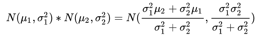
  我们知道正态分布可以这么表示 N(均值，方差)。在我们是用概率分布来计算。所以和直观理解中的计算方式有不同。因为直观理解中的计算方式是相当于粗略估计值这个概率分布的均值与雷达测量值的概率分布的均值进行加权和得到精确估计值的概率分布的均值。由于正态分布是均值那个地方的概率最大，所以当前时刻睿思位置的精确估计值就是它概率分布的均值，既这两个概率分布相乘。公式如下所示：

下面的公式为高斯分布公式：

%matplotlib inline 

import numpy as np

t = np.linspace(1,100,100) # 在1~100s内采样100次
a = 0.5 # 加速度值
position = (a * t**2)/2

position_noise = position+np.random.normal(0,120,size=(t.shape[0])) # 模拟生成GPS位置测量数据（带噪声）
import matplotlib.pyplot as plt
plt.plot(t,position,label='truth position')
plt.plot(t,position_noise,label='only use measured position')


#---------------卡尔曼滤波----------------

predicts = [position_noise[0]]
position_predict = predicts[0]

predict_var = 0
odo_var = 120**2 #这是我们自己设定的位置测量仪器的方差，越大则测量值占比越低
v_std = 50 # 测量仪器的方差（这个方差在现实生活中是需要我们进行传感器标定才能算出来的，可搜Allan方差标定）
for i in range(1,t.shape[0]):
  
    dv =  (position[i]-position[i-1]) + np.random.normal(0,50) # 模拟从IMU读取出的速度
    position_predict = position_predict + dv # 利用上个时刻的位置和速度预测当前位置
    predict_var += v_std**2 # 更新预测数据的方差
    # 下面是Kalman滤波
    position_predict = position_predict*odo_var/(predict_var + odo_var)+position_noise[i]*predict_var/(predict_var + odo_var)
    predict_var = (predict_var * odo_var)/(predict_var + odo_var)
    predicts.append(position_predict)

    
plt.plot(t,predicts,label='kalman filtered position')

plt.legend()
plt.show()

二、匈牙利算法

  匈牙利算法是由匈牙利数学家Edmonds于1965年提出，因而得名。匈牙利算法是基于Hall定理中充分性证明的思想，它是图匹配最常见的算法，该算法的核心就是寻找增广路径，是一种用增广路径求二分图最大匹配的算法。-------大家看到这里是不是一头雾水，看得头大？那么请看下面的版本：

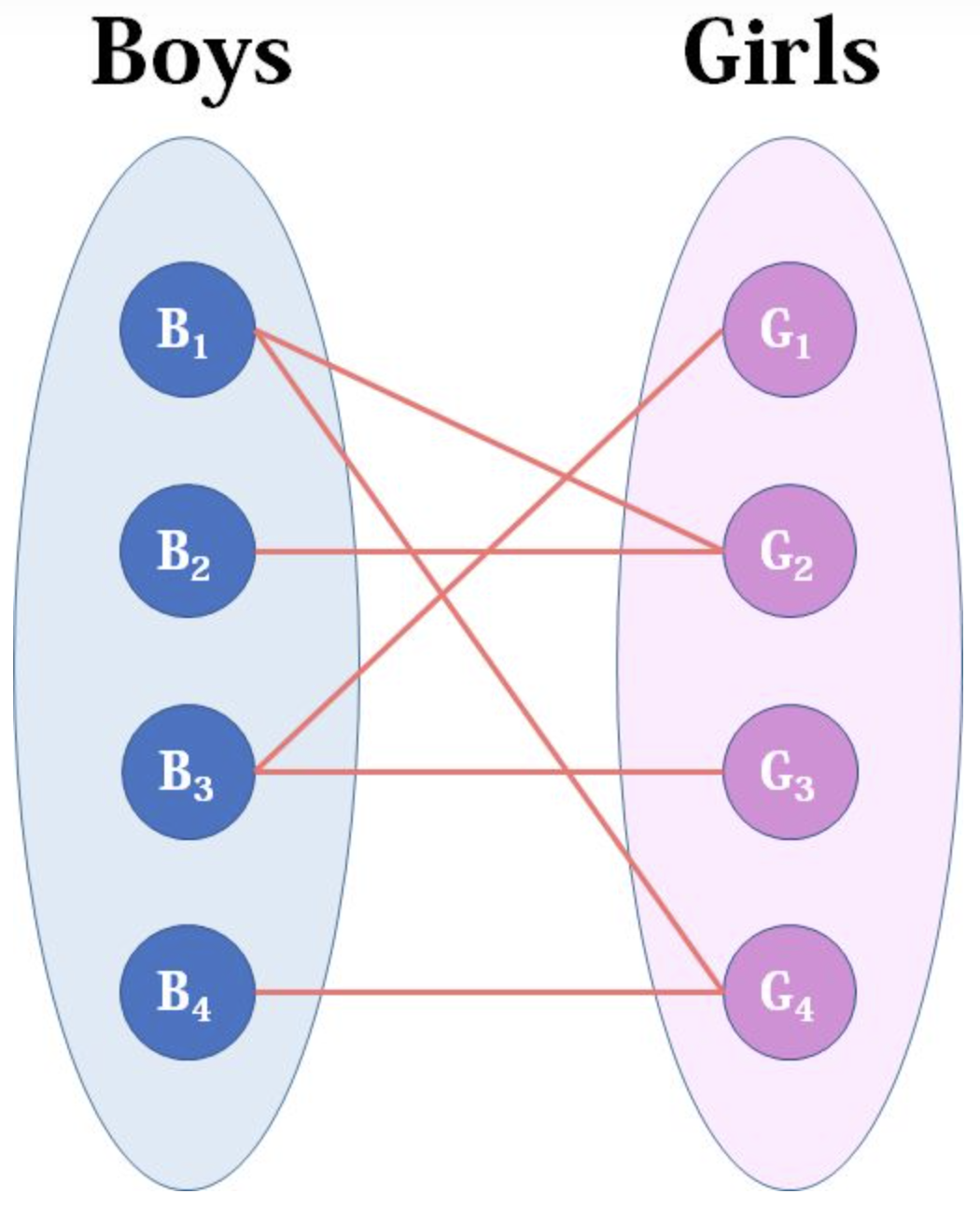
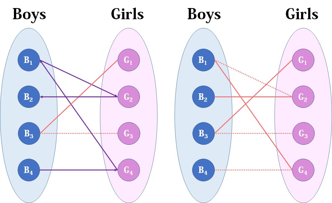
  通过的努力，人类终于可以有了克隆人，睿思克隆了4个自己，找到你，让你帮忙介绍女朋友。所以现在你的手上有4个剩男，假设你正好有4个剩女，每个睿思都可能对多名异性有好感，如果一对男女互有好感，那么你就可以把这一对撮合在一起。你拥有的大概就是下面这样一张关系图，每一条连线都表示互有好感。

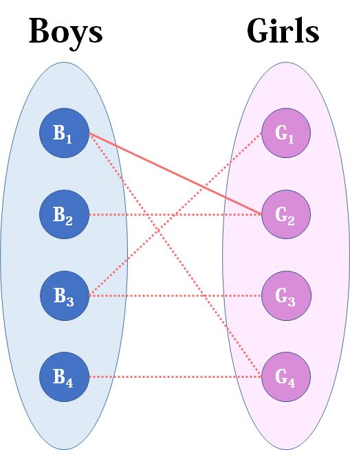
现在我们来看看匈牙利算法是怎么运作的：

我们从1看起（男女平等，从女生这边看起也是可以的），他与G2有暧昧，那我们就先暂时把他与G2连接（注意这时只是你作为一个红娘在纸上构想，你没有真正行动，此时的安排都是暂时的）。

来看2好睿思，2号睿思也喜欢G2，这时G2已经“名花有主”了（虽然只是我们设想的），那怎么办呢？我们倒回去看G2目前被安排的男友，是1号睿思，那么1号睿思有没有别的选项呢？有，G4，G4还没有被安排，那我们就给1号睿思安排上G4。

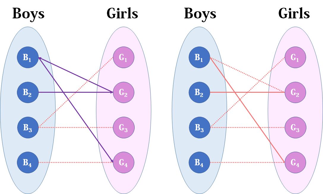
然后3号睿思，3号睿思直接配上G1就好了，这没什么问题。至于4号睿思，他只钟情于G4，G4目前配的是1号睿思。1号睿思除了G4还可以选G2，但是呢，如果1号睿思选了G2，G2的原配2号睿思就没得选了。我们绕了一大圈，发现4号睿思只能注定单身了，可怜。（睿思何苦为难睿思呢）

接下来我们看看匈牙利算法的具体实现

import numpy as np
import collections
import time

class Hungarian():
    """
    """
    def __init__(self, input_matrix=None, is_profit_matrix=False):
        """
        输入为一个二维嵌套列表
        is_profit_matrix=False代表输入是消费矩阵（需要使消费最小化），反之则为利益矩阵（需要使利益最大化）
        """
        if input_matrix is not None:
            # 保存输入
            my_matrix = np.array(input_matrix)
            self._input_matrix = np.array(input_matrix)
            self._maxColumn = my_matrix.shape[1]
            self._maxRow = my_matrix.shape[0]

            # 本算法必须作用于方阵，如果不为方阵则填充0变为方阵
            matrix_size = max(self._maxColumn, self._maxRow)
            pad_columns = matrix_size - self._maxRow
            pad_rows = matrix_size - self._maxColumn
            my_matrix = np.pad(my_matrix, ((0,pad_columns),(0,pad_rows)), 'constant', constant_values=(0))

            # 如果需要，则转化为消费矩阵
            if is_profit_matrix:
                my_matrix = self.make_cost_matrix(my_matrix)

            self._cost_matrix = my_matrix
            self._size = len(my_matrix)
            self._shape = my_matrix.shape

            # 存放算法结果
            self._results = []
            self._totalPotential = 0
        else:
            self._cost_matrix = None
    def make_cost_matrix(self,profit_matrix):
        '''利益矩阵转化为消费矩阵，输出为numpy矩阵'''
        # 消费矩阵 = 利益矩阵最大值组成的矩阵 - 利益矩阵
        matrix_shape = profit_matrix.shape
        offset_matrix = np.ones(matrix_shape, dtype=int) * profit_matrix.max()
        cost_matrix = offset_matrix - profit_matrix
        return cost_matrix
    def get_results(self):
        """获取算法结果"""
        return self._results
    def calculate(self):
        """
        实施匈牙利算法的函数
        """
        result_matrix = self._cost_matrix.copy()

        # 步骤 1: 矩阵每一行减去本行的最小值
        for index, row in enumerate(result_matrix):
            result_matrix[index] -= row.min()

        # 步骤 2: 矩阵每一列减去本行的最小值
        for index, column in enumerate(result_matrix.T):
            result_matrix[:, index] -= column.min()
        #print('步骤2结果 ',result_matrix)
        # 步骤 3： 使用最少数量的划线覆盖矩阵中所有的0元素
        # 如果划线总数不等于矩阵的维度需要进行矩阵调整并重复循环此步骤
        total_covered = 0
        while total_covered < self._size:
            time.sleep(1)
            #print("---------------------------------------")
            #print('total_covered: ',total_covered)
            #print('result_matrix:',result_matrix)
            # 使用最少数量的划线覆盖矩阵中所有的0元素同时记录划线数量
            cover_zeros = CoverZeros(result_matrix)
            single_zero_pos_list = cover_zeros.calculate()
            covered_rows = cover_zeros.get_covered_rows()
            covered_columns = cover_zeros.get_covered_columns()
            total_covered = len(covered_rows) + len(covered_columns)

            # 如果划线总数不等于矩阵的维度需要进行矩阵调整（需要使用未覆盖处的最小元素）
            if total_covered < self._size:
                result_matrix = self._adjust_matrix_by_min_uncovered_num(result_matrix, covered_rows, covered_columns)
        #元组形式结果对存放到列表
        self._results = single_zero_pos_list
        # 计算总期望结果
        value = 0
        for row, column in single_zero_pos_list:
            value += self._input_matrix[row, column]
        self._totalPotential = value

    def get_total_potential(self):
        return self._totalPotential

    def _adjust_matrix_by_min_uncovered_num(self, result_matrix, covered_rows, covered_columns):
        """计算未被覆盖元素中的最小值（m）,未被覆盖元素减去最小值m,行列划线交叉处加上最小值m"""
        adjusted_matrix = result_matrix
        # 计算未被覆盖元素中的最小值（m）
        elements = []
        for row_index, row in enumerate(result_matrix):
            if row_index not in covered_rows:
                for index, element in enumerate(row):
                    if index not in covered_columns:
                        elements.append(element)
        min_uncovered_num = min(elements)
        #print('min_uncovered_num:',min_uncovered_num)
        #未被覆盖元素减去最小值m
        for row_index, row in enumerate(result_matrix):
            if row_index not in covered_rows:
                for index, element in enumerate(row):
                    if index not in covered_columns:
                        adjusted_matrix[row_index,index] -= min_uncovered_num
        #print('未被覆盖元素减去最小值m',adjusted_matrix)
    
        #行列划线交叉处加上最小值m
        for row_ in covered_rows:
            for col_ in covered_columns:
                #print((row_,col_))
                adjusted_matrix[row_,col_] += min_uncovered_num
        #print('行列划线交叉处加上最小值m',adjusted_matrix)

        return adjusted_matrix



class CoverZeros():
    """
    使用最少数量的划线覆盖矩阵中的所有零
    输入为numpy方阵
    """
    def __init__(self, matrix):
        # 找到矩阵中零的位置（输出为同维度二值矩阵，0位置为true，非0位置为false）
        self._zero_locations = (matrix == 0)
        self._zero_locations_copy = self._zero_locations.copy()
        self._shape = matrix.shape

        # 存储划线盖住的行和列
        self._covered_rows = []
        self._covered_columns = []

    def get_covered_rows(self):
        """返回覆盖行索引列表"""
        return self._covered_rows

    def get_covered_columns(self):
        """返回覆盖列索引列表"""
        return self._covered_columns

    def row_scan(self,marked_zeros):
        '''扫描矩阵每一行，找到含0元素最少的行，对任意0元素标记（独立零元素），划去标记0元素（独立零元素）所在行和列存在的0元素'''
        min_row_zero_nums = [9999999,-1]
        for index, row in enumerate(self._zero_locations_copy):#index为行号
            row_zero_nums = collections.Counter(row)[True]
            if row_zero_nums < min_row_zero_nums[0] and row_zero_nums!=0:
                #找最少0元素的行
                min_row_zero_nums = [row_zero_nums,index]
        #最少0元素的行
        row_min = self._zero_locations_copy[min_row_zero_nums[1],:]
        #找到此行中任意一个0元素的索引位置即可
        row_indices, = np.where(row_min)
        #标记该0元素
        #print('row_min',row_min)
        marked_zeros.append((min_row_zero_nums[1],row_indices[0]))
        #划去该0元素所在行和列存在的0元素
        #因为被覆盖，所以把二值矩阵_zero_locations中相应的行列全部置为false
        self._zero_locations_copy[:,row_indices[0]] = np.array([False for _ in range(self._shape[0])])
        self._zero_locations_copy[min_row_zero_nums[1],:] = np.array([False for _ in range(self._shape[0])])

    def calculate(self):
        '''进行计算'''
        #储存勾选的行和列
        ticked_row   = []
        ticked_col   = []
        marked_zeros = []
        #1、试指派并标记独立零元素
        while True:
            #print('_zero_locations_copy',self._zero_locations_copy)
            #循环直到所有零元素被处理（_zero_locations中没有true）
            if True not in self._zero_locations_copy:
                break
            self.row_scan(marked_zeros)
            
        #2、无被标记0（独立零元素）的行打勾
        independent_zero_row_list = [pos[0] for pos in marked_zeros]
        ticked_row = list(set(range(self._shape[0])) - set(independent_zero_row_list))
        #重复3,4直到不能再打勾
        TICK_FLAG = True
        while TICK_FLAG:
            #print('ticked_row:',ticked_row,'   ticked_col:',ticked_col)
            TICK_FLAG = False
            #3、对打勾的行中所含0元素的列打勾
            for row in ticked_row:
                #找到此行
                row_array = self._zero_locations[row,:]
                #找到此行中0元素的索引位置
                for i in range(len(row_array)):
                    if row_array[i] == True and i not in ticked_col:
                        ticked_col.append(i)
                        TICK_FLAG = True
            
            #4、对打勾的列中所含独立0元素的行打勾
            for row,col in marked_zeros:
                if col in ticked_col and row not in ticked_row:
                    ticked_row.append(row)
                    FLAG = True
        #对打勾的列和没有打勾的行画画线
        self._covered_rows    = list(set(range(self._shape[0])) - set(ticked_row))
        self._covered_columns = ticked_col
            



        return marked_zeros



if __name__ == '__main__':
    #以下为3个测试用例
    cost_matrix = [
        [4, 2, 8],
        [4, 3, 7],
        [3, 1, 6]]
    hungarian = Hungarian(cost_matrix)
    print('calculating...')
    hungarian.calculate()
    print("Expected value:\t\t12")
    print("Calculated value:\t", hungarian.get_total_potential())  # = 12
    print("Expected results:\n\t[(0, 1), (1, 0), (2, 2)]")
    print("Results:\n\t", hungarian.get_results())
    print("-" * 80)

    profit_matrix = [
        [62, 75, 80, 93, 95, 97],
        [75, 80, 82, 85, 71, 97],
        [80, 75, 81, 98, 90, 97],
        [78, 82, 84, 80, 50, 98],
        [90, 85, 85, 80, 85, 99],
        [65, 75, 80, 75, 68, 96]]

    hungarian = Hungarian(profit_matrix, is_profit_matrix=True)
    hungarian.calculate()
    print("Expected value:\t\t543")
    print("Calculated value:\t", hungarian.get_total_potential())  # = 543
    print("Expected results:\n\t[(0, 4), (2, 3), (5, 5), (4, 0), (1, 1), (3, 2)]")
    print("Results:\n\t", hungarian.get_results())
    print("-" * 80)
    profit_matrix = [
        [62, 75, 80, 93, 0, 97],
        [75, 0, 82, 85, 71, 97],
        [80, 75, 81, 0, 90, 97],
        [78, 82, 0, 80, 50, 98],
        [0, 85, 85, 80, 85, 99],
        [65, 75, 80, 75, 68, 0]]
    hungarian = Hungarian(profit_matrix, is_profit_matrix=True)
    hungarian.calculate()
    print("Expected value:\t\t523")
    print("Calculated value:\t", hungarian.get_total_potential())  # = 523
    print("Expected results:\n\t[(0, 3), (2, 4), (3, 0), (5, 2), (1, 5), (4, 1)]")
    print("Results:\n\t", hungarian.get_results())
    print("-" * 80)

calculating...
Expected value:		12
Calculated value:	 12
Expected results:
	[(0, 1), (1, 0), (2, 2)]
Results:
	 [(0, 0), (1, 2), (2, 1)]
--------------------------------------------------------------------------------
Expected value:		543
Calculated value:	 543
Expected results:
	[(0, 4), (2, 3), (5, 5), (4, 0), (1, 1), (3, 2)]
Results:
	 [(0, 4), (2, 3), (5, 5), (1, 1), (3, 2), (4, 0)]
--------------------------------------------------------------------------------
Expected value:		523
Calculated value:	 523
Expected results:
	[(0, 3), (2, 4), (3, 0), (5, 2), (1, 5), (4, 1)]
Results:
	 [(0, 3), (2, 4), (3, 0), (1, 5), (4, 1), (5, 2)]
--------------------------------------------------------------------------------

上面的代码为匈牙利算法的实现，这样写的原因是能够帮助大家理解该算法，在Python中，匈牙利算法有更加快速的实现。

from scipy.optimize import linear_sum_assignment
cost =np.array([[4,1,3],[2,0,5],[3,2,2]])
row_ind,col_ind=linear_sum_assignment(cost)
print(row_ind)#开销矩阵对应的行索引
print(col_ind)#对应行索引的最优指派的列索引
print(cost[row_ind,col_ind])#提取每个行索引的最优指派列索引所在的元素，形成数组
print(cost[row_ind,col_ind].sum())#数组求和　　输出：[0 1 2][1 0 2] [1 2 2] 5

[0 1 2]
[1 0 2]
[1 2 2]
5

总结

本次项目中，为大家通俗的介绍了卡尔曼滤波算法以及匈牙利算法，并给出了算法对应的Python实现，通过本项目，大家能够快速入门多目标追踪。