Paddle可视化神经网络热力图(CAM)

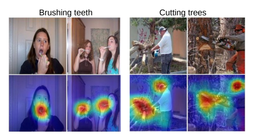
Class Activation Mapping(CAM)是一个帮助可视化CNN的工具，通过它我们可以观察为了达到正确分类的目的，网络更侧重于哪块区域。比如，下面两幅图，一个是刷牙，一个是砍树，我们根据热力图可以看到高响应区域的确集中在我们认为最有助于作出判断的部位。

本项目最初还是来自于项目：讯飞农作物生长情况识别挑战赛baseline(非官方)，因为数据集不大，尽管模型收敛很好，但线上的分数确始终不能更进一步。于是想到可以可视化一下网络的CAM，观察一下指导分类的高响应区域是否落在目标核心部位上。

CAM论文链接地址

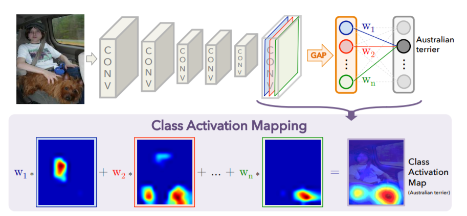
• CAM原理

其计算方法如下图所示。对于一个CNN模型，对其最后一个featuremap做全局平均池化（GAP）计算各通道均值，然后通过FC层等映射到class score，找出argmax，计算最大的那一类的输出相对于最后一个featuremap的梯度，再把这个梯度可视化到原图上即可。直观来说，就是看一下网络抽取到的高层特征的哪部分对最终的classifier影响更大。

!cd 'data/data106772' && unzip -q img.zip

%matplotlib inline
import os
from PIL import Image
import paddle
import numpy as np
import cv2
import matplotlib.pyplot as plt
from draw_features import Res2Net_vd
import paddle.nn.functional as F
import paddle
import warnings
warnings.filterwarnings('ignore')

def draw_CAM(model, img_path, save_path, transform=None, visual_heatmap=False):
    '''
    绘制 Class Activation Map
    :param model: 加载好权重的Pytorch model
    :param img_path: 测试图片路径
    :param save_path: CAM结果保存路径
    :param transform: 输入图像预处理方法
    :param visual_heatmap: 是否可视化原始heatmap（调用matplotlib）
    :return:
    '''
    # 图像加载&预处理
    img = Image.open(img_path).convert('RGB')
    img = img.resize((224, 224), Image.BILINEAR) #Image.BILINEAR双线性插值
    if transform:
        img = transform(img)
    # img = img.unsqueeze(0)
    img = np.array(img).astype('float32')
    img = img.transpose((2, 0, 1))
    img = paddle.to_tensor(img)
    img = paddle.unsqueeze(img, axis=0)
    # print(img.shape)
    # 获取模型输出的feature/score

    output,features = model(img)

    print('outputshape:',output.shape)
    print('featureshape:',features.shape)
    # lab = np.argmax(out.numpy())
    # 为了能读取到中间梯度定义的辅助函数
    def extract(g):
        global features_grad
        features_grad = g
 
    # 预测得分最高的那一类对应的输出score
    pred = np.argmax(output.numpy())
    # print('***********pred:',pred)
    pred_class = output[:, pred]
    # print(pred_class)

    features.register_hook(extract)
    pred_class.backward() # 计算梯度
 
    grads = features_grad   # 获取梯度
    # print(grads.shape)
    # pooled_grads = paddle.nn.functional.adaptive_avg_pool2d( x = grads, output_size=[1, 1])
    pooled_grads = grads
    
    # 此处batch size默认为1，所以去掉了第0维（batch size维）
    pooled_grads = pooled_grads[0]
    # print('pooled_grads:', pooled_grads.shape)
    # print(pooled_grads.shape)
    features = features[0]

    # print(features.shape)
    # 最后一层feature的通道数
    for i in range(2048):
        features[i, ...] *= pooled_grads[i, ...]
 
    heatmap = features.detach().numpy()
    
    heatmap = np.mean(heatmap, axis=0)
    # print(heatmap)
    heatmap = np.maximum(heatmap, 0)
    # print('+++++++++',heatmap)
    heatmap /= np.max(heatmap)
    # print('+++++++++',heatmap)
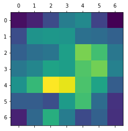
    # 可视化原始热力图
    if visual_heatmap:
        plt.matshow(heatmap)
        plt.show()
 
    img = cv2.imread(img_path)  # 用cv2加载原始图像
    heatmap = cv2.resize(heatmap, (img.shape[1], img.shape[0]))  # 将热力图的大小调整为与原始图像相同
    heatmap = np.uint8(255 * heatmap)  # 将热力图转换为RGB格式
    # print(heatmap.shape)
    heatmap = cv2.applyColorMap(heatmap, cv2.COLORMAP_JET)  # 将热力图应用于原始图像
    superimposed_img = heatmap * 0.4 + img  # 这里的0.4是热力图强度因子
    cv2.imwrite(save_path, superimposed_img)  # 将图像保存到硬盘


model_re2 = Res2Net_vd(layers=50, scales=4, width=26, class_dim=4)
# model_re2 = Res2Net50_vd_26w_4s(class_dim=4)
modelre2_state_dict = paddle.load("Hapi_MyCNN.pdparams")
model_re2.set_state_dict(modelre2_state_dict, use_structured_name=True)
use_gpu = True

paddle.set_device('gpu:0') if use_gpu else paddle.set_device('cpu')

model_re2.eval()

gpu = True

paddle.set_device('gpu:0') if use_gpu else paddle.set_device('cpu')

model_re2.eval()

draw_CAM(model_re2, 'data/data106772/img/test/629.jpg', 'test3.jpg', transform=None, visual_heatmap=True)

W1123 17:02:34.611114  6534 device_context.cc:447] Please NOTE: device: 0, GPU Compute Capability: 7.0, Driver API Version: 10.1, Runtime API Version: 10.1
W1123 17:02:34.615968  6534 device_context.cc:465] device: 0, cuDNN Version: 7.6.


outputshape: [1, 4]
featureshape: [1, 2048, 7, 7]

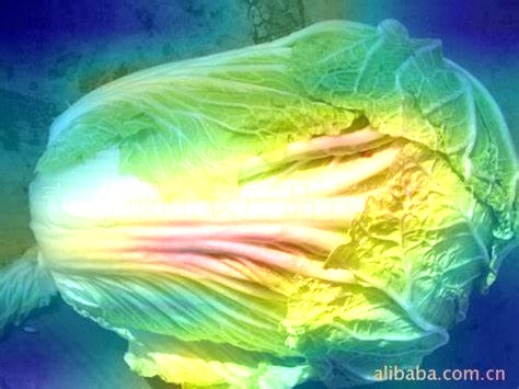
• 实验结果

• 代码详解

关于代码，相信注释已经写得很明白了，需要注意的是，我把网络结构多返回了softmax层之前的特征向量，代码如下所示：

    def forward(self, inputs):
        y = self.conv1_1(inputs)
        y = self.conv1_2(y)
        y = self.conv1_3(y)
        y = self.pool2d_max(y)
        blocks = []
        for block in self.block_list:
            y = block(y)
            blocks.append(y)
        # draw_features(32, 32, y.cpu().numpy(), "{}/f7_layer3.png".format(savepath))
        # y = self.convf_1(y)
        y = self.pool2d_avg(y)
        y = paddle.reshape(y, shape=[-1, self.pool2d_avg_channels])
        out = self.out(y)
        blocks.append(out)
        return blocks[-1:-3:-1]

总结

通过该可视化方法，可以有针对性的对数据集进行扩充，以此来指导数据增强的方向。需要注意的是，大家需要对网络结构足够了解，CAM主要使用最后一层的特征向量，大家注意区分。