
【目标检测入门教程】基于飞桨实现单发多框检测(SSD)
单发多框检测(SSD)模型简单、快速且被广泛使用。尽管这只是其中一种目标检测模型,但其中的一些设计原则和实现细节也适用于其他模型。
基于飞桨实现单发多框检测(SSD)
单发多框检测(SSD)模型简单、快速且被广泛使用。尽管这只是其中一种目标检测模型,但其中的一些设计原则和实现细节也适用于其他模型。
参考资料:
- 《动手学深度学习》第二版:
http://zh.d2l.ai/chapter_computer-vision/ssd.html - 从图像分类开始带你快速了解计算机视觉的目标检测任务:https://aistudio.baidu.com/aistudio/projectdetail/1753617
一、模型
单发多框检测模型的设计如下图所示。 此模型主要由基础网络组成,其后是几个多尺度特征块。 基本网络用于从输入图像中提取特征,因此它可以使用深度卷积神经网络。 单发多框检测论文中选用了在分类层之前截断的VGG,现在也常用ResNet替代。 我们可以设计基础网络,使它输出的高和宽较大。 这样一来,基于该特征图生成的锚框数量较多,可以用来检测尺寸较小的目标。 接下来的每个多尺度特征块将上一层提供的特征图的高和宽缩小(如减半),并使特征图中每个单元在输入图像上的感受野变得更广阔。

通过深度神经网络分层表示图像的多尺度目标检测的设计。 由于接近顶部的多尺度特征图较小,但具有较大的感受野,它们适合检测较少但较大的物体。 简而言之,通过多尺度特征块,单发多框检测生成不同大小的锚框,并通过预测边界框的类别和偏移量来检测大小不同的目标,因此这是一个多尺度目标检测模型。
为了运行本项目代码,首先导入必要的资源库:
%matplotlib inline
from matplotlib import pyplot as plt
import paddle
from paddle import nn
from paddle.nn import functional as F
1.类别预测层
设目标的类别个数为 q q q。每个锚框的类别个数将是 q + 1 q+1 q+1,其中类别0表示锚框只包含背景。在某个尺度下,设特征图的高和宽分别为 h h h和 w w w,如果以其中每个单元为中心生成 a a a个锚框,那么我们需要对 h ∗ w ∗ a h*w*a h∗w∗a个锚框进行分类。如果使用全连接层作为输出,很容易导致模型参数过多。为了解决这一问题,我们可以使用卷积层的通道来输出类别预测的方法,以此来降低模型复杂度。
具体来说,类别预测层使用一个保持输入高和宽的卷积层。这样一来,输出和输入在特征图宽和高上的空间坐标一一对应。考虑输出和输入同一空间坐标 ( x , y ) (x,y) (x,y):输出特征图上 ( x , y ) (x,y) (x,y)坐标的通道里包含了以输入特征图 ( x , y ) (x,y) (x,y)坐标为中心生成的所有锚框的类别预测。因此输出通道数为 a ( q + 1 ) a(q+1) a(q+1),其中索引为 i ( q + 1 ) + j i(q+1) + j i(q+1)+j( 0 ≤ j ≤ q 0 \leq j \leq q 0≤j≤q)的通道代表了索引为 i i i的锚框有关类别索引为 j j j的预测。
下面我们定义一个这样的类别预测层:指定参数 a a a和 q q q后,它使用一个填充为1的 3 × 3 3\times3 3×3卷积层。该卷积层的输入和输出的高和宽保持不变。
def cls_predictor(num_inputs, num_anchors, num_classes):
    return nn.Conv2D(num_inputs, num_anchors * (num_classes + 1),
                     kernel_size=5, padding=2)
2.边界框预测层
边界框预测层的设计与类别预测层的设计类似。唯一不同的是,这里需要为每个锚框预测4个偏移量,而不是 q + 1 q+1 q+1个类别。
def bbox_predictor(num_inputs, num_anchors):
    return nn.Conv2D(num_inputs, num_anchors * 4, kernel_size=5, padding=2)
3.连结多尺度的预测
前面提到,单发多框检测根据多个尺度下的特征图生成锚框并预测类别和偏移量。由于每个尺度上特征图的形状或以同一单元为中心生成的锚框个数都可能不同,因此不同尺度的预测输出形状可能不同。
在下面的例子中,我们对同一批量数据构造两个不同尺度下的特征图Y1和Y2,其中Y2相对于Y1来说高和宽分别减半。以类别预测为例,假设以Y1和Y2特征图中每个单元生成的锚框个数分别是5和3,当目标类别个数为10时,类别预测输出的通道数分别为 5 × ( 10 + 1 ) = 55 5\times(10+1)=55 5×(10+1)=55和 3 × ( 10 + 1 ) = 33 3\times(10+1)=33 3×(10+1)=33。预测输出的格式为(批量大小, 通道数, 高, 宽)。可以看到,除了批量大小外,其他维度大小均不一样。我们需要将它们变形成统一的格式并将多尺度的预测连结,从而让后续计算更简单。
def forward(x, block):
    return block(x)

Y1 = forward(paddle.zeros(shape=[2, 8, 20, 20]), cls_predictor(8, 5, 10))
Y2 = forward(paddle.zeros(shape=[2, 16, 10, 10]), cls_predictor(16, 3, 10))
Y1.shape, Y2.shape
([2, 55, 20, 20], [2, 33, 10, 10])
正如我们所看到的,除了批量大小这一维度外,其他三个维度都具有不同的尺寸。 为了将这两个预测输出链接起来以提高计算效率,我们将把这些张量转换为更一致的格式。
通道维包含中心相同的锚框的预测结果。我们首先将通道维移到最后一维。因为不同尺度下批量大小仍保持不变,我们可以将预测结果转成二维的(批量大小, 高 × \times ×宽 × \times ×通道数)的格式,以方便之后在维度1上的连结。
def flatten_pred(pred):
    return paddle.flatten(paddle.transpose(pred, perm=[0, 2, 3, 1]), start_axis=1)

def concat_preds(preds):
    return paddle.concat([flatten_pred(p) for p in preds], axis=-1)
这样一来,尽管Y1和Y2形状不同,我们仍然可以将这两个同一批量不同尺度的预测结果连结在一起。
concat_preds([Y1, Y2]).shape
[2, 25300]
4.高和宽减半块
为了在多尺度检测目标,下面定义高和宽减半块down_sample_blk。它串联了两个填充为1的 3 × 3 3\times3 3×3卷积层和步幅为2的 2 × 2 2\times2 2×2最大池化层。我们知道,填充为1的 3 × 3 3\times3 3×3卷积层不改变特征图的形状,而后面的池化层则直接将特征图的高和宽减半。由于 1 × 2 + ( 3 − 1 ) + ( 3 − 1 ) = 6 1\times 2+(3-1)+(3-1)=6 1×2+(3−1)+(3−1)=6,输出特征图中每个单元在输入特征图上的感受野形状为 6 × 6 6\times6 6×6。可以看出,高和宽减半块使输出特征图中每个单元的感受野变得更广阔。
def down_sample_blk(in_channels, out_channels):
    blk = []
    for _ in range(2):
        blk.append(nn.Conv2D(in_channels, out_channels,
                             kernel_size=3, padding=1))
        blk.append(nn.BatchNorm2D(out_channels))
        blk.append(nn.ReLU())
        in_channels = out_channels
    blk.append(nn.MaxPool2D(2))
    return nn.Sequential(*blk)
在以下示例中,我们构建的高和宽减半块会更改输入通道的数量,并将输入特征图的高度和宽度减半。
forward(paddle.zeros((2, 3, 20, 20)), down_sample_blk(3, 10)).shape
[2, 10, 10, 10]
5.基础网络块
基础网络块用来从原始图像中抽取特征。为了计算简洁,我们在这里构造一个小的基础网络。该网络串联3个高和宽减半块,并逐步将通道数翻倍。当输入的原始图像的形状为 256 × 256 256\times256 256×256时,基础网络块输出的特征图的形状为 32 × 32 32 \times 32 32×32。
def base_net():
    blk = []
    num_filters = [3, 16, 32, 64]
    for i in range(len(num_filters) - 1):
        blk.append(down_sample_blk(num_filters[i], num_filters[i+1]))
    return nn.Sequential(*blk)

forward(paddle.zeros((2, 3, 256, 256)), base_net()).shape
[2, 64, 32, 32]
6.完整的模型
单发多框检测模型一共包含5个模块,每个模块输出的特征图既用来生成锚框,又用来预测这些锚框的类别和偏移量。第一模块为基础网络块,第二模块至第四模块为高和宽减半块,第五模块使用全局最大池化层将高和宽降到1。因此第二模块至第五模块均为多尺度特征块。
def get_blk(i):
    if i == 0:
        blk = base_net()
    elif i == 1:
        blk = down_sample_blk(64, 128)
    elif i == 4:
        blk = nn.AdaptiveMaxPool2D((1,1))
    else:
        blk = down_sample_blk(128, 128)
    return blk
接下来,我们定义每个模块如何进行前向计算。跟之前介绍的卷积神经网络不同,这里不仅返回卷积计算输出的特征图Y,还返回根据Y生成的当前尺度的锚框,以及基于Y预测的锚框类别和偏移量。
def box_corner_to_center(boxes):
    """Convert from (upper_left, bottom_right) to (center, width, height)"""
    x1, y1, x2, y2 = boxes[:, 0], boxes[:, 1], boxes[:, 2], boxes[:, 3]
    cx = (x1 + x2) / 2
    cy = (y1 + y2) / 2
    w = x2 - x1
    h = y2 - y1
    boxes = paddle.stack((cx, cy, w, h), axis=-1)
    return boxes

def box_center_to_corner(boxes):
    """Convert from (center, width, height) to (upper_left, bottom_right)"""
    cx, cy, w, h = boxes[:, 0], boxes[:, 1], boxes[:, 2], boxes[:, 3]
    x1 = cx - 0.5 * w
    y1 = cy - 0.5 * h
    x2 = cx + 0.5 * w
    y2 = cy + 0.5 * h
    boxes = paddle.stack((x1, y1, x2, y2), axis=-1)
    return boxes


# Defined in file: ./chapter_computer-vision/bounding-box.md
def bbox_to_rect(bbox, color):
    """Convert bounding box to matplotlib format."""
    # Convert the bounding box (top-left x, top-left y, bottom-right x,
    # bottom-right y) format to matplotlib format: ((upper-left x,
    # upper-left y), width, height)
    return plt.Rectangle(
        xy=(bbox[0], bbox[1]), width=bbox[2]-bbox[0], height=bbox[3]-bbox[1],
        fill=False, edgecolor=color, linewidth=2)


# Defined in file: ./chapter_computer-vision/anchor.md
def multibox_prior(data, sizes, ratios):
    in_height, in_width = data.shape[-2:]
    num_sizes, num_ratios = len(sizes), len(ratios)
    boxes_per_pixel = (num_sizes + num_ratios - 1)
    size_tensor = paddle.to_tensor(sizes)
    ratio_tensor = paddle.to_tensor(ratios)
    # Offsets are required to move the anchor to center of a pixel
    # Since pixel (height=1, width=1), we choose to offset our centers by 0.5
    offset_h, offset_w = 0.5, 0.5
    steps_h = 1.0 / in_height  # Scaled steps in y axis
    steps_w = 1.0 / in_width  # Scaled steps in x axis

    # Generate all center points for the anchor boxes
    center_h = (paddle.arange(in_height) + offset_h) * steps_h
    center_w = (paddle.arange(in_width) + offset_w) * steps_w
    shift_y, shift_x = paddle.meshgrid(center_h, center_w)
    shift_y, shift_x = shift_y.reshape([-1]), shift_x.reshape([-1])

    # Generate boxes_per_pixel number of heights and widths which are later
    # used to create anchor box corner coordinates (xmin, xmax, ymin, ymax)
    # cat (various sizes, first ratio) and (first size, various ratios)
    w = paddle.concat((size_tensor * paddle.sqrt(ratio_tensor[0]),
                   sizes[0] * paddle.sqrt(ratio_tensor[1:])))\
                   * in_height / in_width  # handle rectangular inputs
    h = paddle.concat((size_tensor / paddle.sqrt(ratio_tensor[0]),
                   sizes[0] / paddle.sqrt(ratio_tensor[1:])))
    # Divide by 2 to get half height and half width
    anchor_manipulations = paddle.tile(paddle.t(paddle.stack([-w, -h, w, h])), repeat_times=[in_height * in_width, 1]) /2

    # Each center point will have boxes_per_pixel number of anchor boxes, so
    # generate grid of all anchor box centers with boxes_per_pixel repeats
    out_grid = paddle.tile(paddle.stack([shift_x, shift_y, shift_x, shift_y],
                axis=1), repeat_times=[boxes_per_pixel, 1])

    output = out_grid + anchor_manipulations
    return output.unsqueeze(0)
def blk_forward(X, blk, size, ratio, cls_predictor, bbox_predictor):
    Y = blk(X)
    anchors = multibox_prior(Y, sizes=size, ratios=ratio)
    cls_preds = cls_predictor(Y)
    bbox_preds = bbox_predictor(Y)
    return (Y, anchors, cls_preds, bbox_preds)
回想一下,一个较接近顶部的多尺度特征块是用于检测较大目标的,因此需要生成更大的锚框。
在上面的前向传播中,在每个多尺度特征块上,我们通过调用的multibox_prior函数的sizes参数传递两个比例值的列表。
在下面,0.2和1.05之间的区间被均匀分成五个部分,以确定五个模块的在不同尺度下的较小值:0.2、0.37、0.54、0.71和0.88。
之后,他们较大的值由 0.2 × 0.37 = 0.272 \sqrt{0.2 \times 0.37} = 0.272 0.2×0.37=0.272、 0.37 × 0.54 = 0.447 \sqrt{0.37 \times 0.54} = 0.447 0.37×0.54=0.447等给出。
sizes = [[0.2, 0.272], [0.37, 0.447], [0.54, 0.619], [0.71, 0.79],
         [0.88, 0.961]]
ratios = [[1, 2, 0.5]] * 5
num_anchors = len(sizes[0]) + len(ratios[0]) - 1
现在,我们就可以按如下方式定义完整的模型TinySSD了。
class TinySSD(nn.Layer):
    def __init__(self, num_classes, **kwargs):
        super(TinySSD, self).__init__(**kwargs)
        self.num_classes = num_classes
        idx_to_in_channels = [64, 128, 128, 128, 128]
        for i in range(5):
            # 即赋值语句self.blk_i=get_blk(i)
            setattr(self, f'blk_{i}', get_blk(i))
            setattr(self, f'cls_{i}', cls_predictor(idx_to_in_channels[i],
                                                    num_anchors, num_classes))
            setattr(self, f'bbox_{i}', bbox_predictor(idx_to_in_channels[i],
                                                      num_anchors))

    def forward(self, X):
        anchors, cls_preds, bbox_preds = [None] * 5, [None] * 5, [None] * 5
        for i in range(5):
            # getattr(self,'blk_%d'%i)即访问self.blk_i
            X, anchors[i], cls_preds[i], bbox_preds[i] = blk_forward(
                X, getattr(self, f'blk_{i}'), sizes[i], ratios[i],
                getattr(self, f'cls_{i}'), getattr(self, f'bbox_{i}'))
        anchors = paddle.concat(anchors, axis=1)
        cls_preds = concat_preds(cls_preds)
        cls_preds = cls_preds.reshape([cls_preds.shape[0], -1, self.num_classes + 1])
        bbox_preds = concat_preds(bbox_preds)
        return anchors, cls_preds, bbox_preds
我们创建一个模型实例,然后使用它对一个 256 × 256 256 \times 256 256×256像素的小批量图像X执行前向传播。
如本节前面部分所示,第一个模块输出特征图的形状为 32 × 32 32 \times 32 32×32。
回想一下,第二到第四个模块为高和宽减半块,第五个模块为全局汇聚层。
由于以特征图的每个单元为中心有 4 4 4个锚框生成,因此在所有五个尺度下,每个图像总共生成 ( 3 2 2 + 1 6 2 + 8 2 + 4 2 + 1 ) × 4 = 5444 (32^2 + 16^2 + 8^2 + 4^2 + 1)\times 4 = 5444 (322+162+82+42+1)×4=5444个锚框。
net = TinySSD(num_classes=1)
X = paddle.zeros(shape=[32, 3, 256, 256])
anchors, cls_preds, bbox_preds = net(X)

print('output anchors:', anchors.shape)
print('output class preds:', cls_preds.shape)
print('output bbox preds:', bbox_preds.shape)
output anchors: [1, 5444, 4]
output class preds: [32, 5444, 2]
output bbox preds: [32, 21776]
二、训练模型
现在,我们将描述如何训练用于目标检测的单发多框检测模型。
1.读取数据集和初始化
首先,让我们读取香蕉检测数据集
# 解压数据集
!unzip -oq /home/aistudio/data/data124932/banana-detection.zip
import os
import pandas as pd
import cv2
import numpy as np

def read_data_bananas(is_train=True):
    """Read the bananas dataset images and labels."""
    data_dir = 'banana-detection'
    csv_fname = os.path.join(data_dir, 'bananas_train' if is_train
                                    else 'bananas_val', 'label.csv')
    csv_data = pd.read_csv(csv_fname)
    csv_data = csv_data.set_index('img_name')
    mean = [0.485, 0.456, 0.406]
    std = [0.229, 0.224, 0.225]
    mean = np.array(mean).reshape((1, 1, -1))
    std = np.array(std).reshape((1, 1, -1))
    images, targets = [], []
    for img_name, target in csv_data.iterrows():
        img = cv2.imread(os.path.join(data_dir, 'bananas_train' if is_train else
                         'bananas_val', 'images', f'{img_name}'))
        img = cv2.cvtColor(img, cv2.COLOR_BGR2RGB)
        img = (img / 255.0 - mean) / std # 归一化
        img = img.astype('float32').transpose((2, 0, 1))
        images.append(img)
        # Since all images have same object class i.e. category '0',
        # the `label` column corresponds to the only object i.e. banana
        # The target is as follows : (`label`, `xmin`, `ymin`, `xmax`, `ymax`)
        targets.append(list(target))
    return paddle.to_tensor(images), paddle.to_tensor(targets).unsqueeze(1) / 256

class BananasDataset(paddle.io.Dataset):
    def __init__(self, is_train):
        self.features, self.labels = read_data_bananas(is_train)
        print('read ' + str(len(self.features)) + (f' training examples' if
              is_train else f' validation examples'))

    def __getitem__(self, idx):
        return (self.features[idx], self.labels[idx])

    def __len__(self):
        return len(self.features)

banana =  BananasDataset(is_train=True)
/opt/conda/envs/python35-paddle120-env/lib/python3.7/site-packages/paddle/tensor/creation.py:130: DeprecationWarning: `np.object` is a deprecated alias for the builtin `object`. To silence this warning, use `object` by itself. Doing this will not modify any behavior and is safe.
Deprecated in NumPy 1.20; for more details and guidance: https://numpy.org/devdocs/release/1.20.0-notes.html#deprecations
  if data.dtype == np.object:


read 1000 training examples
加载数据,可视化数据集中某一张图像:
mean = [0.485, 0.456, 0.406]
std = [0.229, 0.224, 0.225]
for data, label in banana:
    image = data.numpy().transpose((1, 2, 0))
    image = cv2.cvtColor(image, cv2.COLOR_BGR2RGB)
    label = label.numpy() * 256
    cv2.rectangle(image, (int(label[0][1]), int(label[0][2])), (int(label[0][3]), int(label[0][4])), (0, 255, 0), 4)
    image = cv2.cvtColor(image, cv2.COLOR_BGR2RGB)
    image = (image * std + mean) * 255.0 # 反归一化
    image = image.astype('int64')
    plt.imshow(image)
    plt.show()
    break
Clipping input data to the valid range for imshow with RGB data ([0..1] for floats or [0..255] for integers).
![[外链图片转存失败,源站可能有防盗链机制,建议将图片保存下来直接上传(img-Hp2mXxzm-1642135952058)(output_35_1.png)]](https://i-blog.csdnimg.cn/blog_migrate/2751c84b60f7349c41de4dcae1c4ca24.png)
检查数据尺寸是否与期望输出一致:
train_loader = paddle.io.DataLoader(banana, batch_size=32, shuffle=True)
for batch_id, data in enumerate(train_loader()):
    x_data = data[0]
    y_data = data[1]

    print("image shape:{}".format(x_data.shape))
    print("label shape:{}".format(y_data.shape))
    break
image shape:[32, 3, 256, 256]
label shape:[32, 1, 5]
香蕉检测数据集中,目标的类别数为1。 定义好模型后,我们需要初始化其参数并定义优化算法。
net = TinySSD(num_classes=1)
trainer = paddle.optimizer.SGD(learning_rate=0.1, parameters=net.parameters(), weight_decay=5e-4)
2.定义损失函数和评价函数
目标检测有两种类型的损失。
第一种有关锚框类别的损失:我们可以简单地复用之前图像分类问题里一直使用的交叉熵损失函数来计算;
第二种有关正类锚框偏移量的损失:预测偏移量是一个回归问题。
但是,对于这个回归问题,我们在这里不使用平方损失,而是使用 L 1 L_1 L1范数损失,即预测值和真实值之差的绝对值。
掩码变量bbox_masks令负类锚框和填充锚框不参与损失的计算。
最后,我们将锚框类别和偏移量的损失相加,以获得模型的最终损失函数。
cls_loss = nn.CrossEntropyLoss()
bbox_loss = nn.L1Loss()

def calc_loss(cls_preds, cls_labels, bbox_preds, bbox_labels, bbox_masks):
    batch_size, num_classes = cls_preds.shape[0], cls_preds.shape[2]
    cls = cls_loss(cls_preds.reshape([-1, num_classes]), cls_labels.reshape([-1]))
    bbox = bbox_loss(bbox_preds * bbox_masks,
                     bbox_labels * bbox_masks)
    return cls + bbox
我们可以使用准确率评价分类结果。
由于偏移量使用了 L 1 L_1 L1范数损失,我们使用平均绝对误差来评价边界框的预测结果。这些预测结果是从生成的锚框及其预测偏移量中获得的。
def cls_eval(cls_preds, cls_labels):
    # 由于类别预测结果放在最后一维,argmax需要指定最后一维。
    return float((cls_preds.argmax(axis=-1) == cls_labels).sum())

def bbox_eval(bbox_preds, bbox_labels, bbox_masks):
    return float((paddle.abs((bbox_labels - bbox_preds) * bbox_masks)).sum())
3.训练模型
在训练模型时,我们需要在模型的前向传播过程中生成多尺度锚框(anchors),并预测其类别(cls_preds)和偏移量(bbox_preds)。
然后,我们根据标签信息Y为生成的锚框标记类别(cls_labels)和偏移量(bbox_labels)。
最后,我们根据类别和偏移量的预测和标注值计算损失函数。为了代码简洁,这里没有评价测试数据集。
def box_iou(boxes1, boxes2):
    boxes1, boxes2 = np.array(boxes1), np.array(boxes2)
    lt = np.maximum(boxes1[:, None, :2], boxes2[:, :2])
    rb = np.minimum(boxes1[:, None, 2:], boxes2[:, 2:])
    wh = np.maximum(rb - lt + 1, 0)
    inter = wh[:, :, 0] * wh[:, :, 1]
    areas1 = (boxes1[:, 2] - boxes1[:, 0] + 1) * (boxes1[:, 3] - boxes1[:, 1] + 1)
    areas2 = (boxes2[:, 2] - boxes2[:, 0] + 1) * (boxes2[:, 3] - boxes2[:, 1] + 1)
    iou = inter / (areas1[:, None] + areas2 - inter)
    return paddle.to_tensor(iou)

def match_anchor_to_bbox(ground_truth, anchors, iou_threshold=0.5):
    """Assign ground-truth bounding boxes to anchor boxes similar to them."""
    num_anchors, num_gt_boxes = anchors.shape[0], ground_truth.shape[0]
    # Element `x_ij` in the `i^th` row and `j^th` column is the IoU
    # of the anchor box `anc_i` to the ground-truth bounding box `box_j`
    jaccard = box_iou(anchors, ground_truth)
    # Initialize the tensor to hold assigned ground truth bbox for each anchor
    anchors_bbox_map = paddle.full((num_anchors,), -1, dtype="int64")
    # Assign ground truth bounding box according to the threshold
    max_ious = paddle.max(jaccard)
    indices = paddle.argmax(jaccard)
    anc_i = paddle.nonzero(max_ious >= 0.5)
    box_j = indices[0]
    anchors_bbox_map[anc_i] = box_j
    # Find the largest iou for each bbox
    col_discard = paddle.full((num_anchors,), -1)
    row_discard = paddle.full((num_gt_boxes,), -1)
    for _ in range(num_gt_boxes):
        max_idx = paddle.argmax(jaccard)
        box_idx = paddle.cast(max_idx % num_gt_boxes, dtype='int64')# (max_idx % num_gt_boxes)#.long()
        anc_idx = paddle.cast(max_idx / num_gt_boxes, dtype='int64')# (max_idx / num_gt_boxes)#.long()
        anchors_bbox_map[anc_idx] = box_idx
    return anchors_bbox_map

def offset_boxes(anchors, assigned_bb, eps=1e-6):
    c_anc = box_corner_to_center(anchors)
    c_assigned_bb = box_corner_to_center(assigned_bb)
    offset_xy = 10 * (c_assigned_bb[:, :2] - c_anc[:, :2]) / c_anc[:, 2:]
    offset_wh = 5 * paddle.log(eps + c_assigned_bb[:, 2:] / c_anc[:, 2:])
    offset = paddle.concat([offset_xy, offset_wh], axis=1)
    return offset

def multibox_target(anchors, labels):
    batch_size, anchors = labels.shape[0], anchors.squeeze(0)
    batch_offset, batch_mask, batch_class_labels = [], [], []
    num_anchors = anchors.shape[0]
    for i in range(batch_size):
        label = labels[i, :, :]
        anchors_bbox_map = match_anchor_to_bbox(label[:, 1:], anchors)
        bbox_mask = (paddle.cast((anchors_bbox_map >= 0), dtype='float64').unsqueeze(-1))
        bbox_mask = paddle.tile(bbox_mask, repeat_times=[1, 4])
        # Initialize class_labels and assigned bbox coordinates with zeros
        class_labels = paddle.zeros([num_anchors], dtype="int64")
        assigned_bb = paddle.zeros([num_anchors, 4], dtype="float32")
        # Assign class labels to the anchor boxes using matched gt bbox labels
        # If no gt bbox is assigned to an anchor box, then let the
        # class_labels and assigned_bb remain zero, i.e the background class
        indices_true = paddle.nonzero(anchors_bbox_map >= 0)
        bb_idx = anchors_bbox_map[indices_true]
        class_labels[indices_true] = paddle.cast(label[0][0], dtype="int64") + 1
        assigned_bb[indices_true] = label[0][1:]
        # offset transformations
        offset = offset_boxes(anchors, assigned_bb) * bbox_mask
        batch_offset.append(offset.reshape([-1]))
        batch_mask.append(bbox_mask.reshape([-1]))
        batch_class_labels.append(class_labels)
    bbox_offset = paddle.stack(batch_offset)
    bbox_mask = paddle.stack(batch_mask)
    class_labels = paddle.stack(batch_class_labels)
    return (bbox_offset, bbox_mask, class_labels)

class Accumulator:
    """For accumulating sums over `n` variables."""
    def __init__(self, n):
        self.data = [0.0] * n

    def add(self, *args):
        self.data = [a + float(b) for a, b in zip(self.data, args)]

    def reset(self):
        self.data = [0.0] * len(self.data)

    def __getitem__(self, idx):
        return self.data[idx]
num_epochs = 20

for epoch in range(num_epochs):
    # 训练精确度的和,训练精确度的和中的示例数
    # 绝对误差的和,绝对误差的和中的示例数
    metric = Accumulator(4)
    net.train()
    for i, (features, target) in enumerate(train_loader()):
        trainer.clear_grad()
        X, Y = features, target
        # 生成多尺度的锚框,为每个锚框预测类别和偏移量
        anchors, cls_preds, bbox_preds = net(X)
        # 为每个锚框标注类别和偏移量
        bbox_labels, bbox_masks, cls_labels = multibox_target(anchors, Y)
        # 根据类别和偏移量的预测和标注值计算损失函数
        l = calc_loss(cls_preds, cls_labels, bbox_preds, bbox_labels, bbox_masks)
        l.mean().backward()
        trainer.step()
        metric.add(cls_eval(cls_preds, cls_labels), cls_labels.numel(),
                   bbox_eval(bbox_preds, bbox_labels, bbox_masks),
                   bbox_labels.numel())
    cls_err, bbox_mae = 1 - metric[0] / metric[1], metric[2] / metric[3]
    print(f'epoch: {epoch}, loss: {l.mean().numpy()[0]}, class err: {cls_err:.2e}, bbox mae: {bbox_mae:.2e}')
/opt/conda/envs/python35-paddle120-env/lib/python3.7/site-packages/paddle/nn/layer/norm.py:653: UserWarning: When training, we now always track global mean and variance.
  "When training, we now always track global mean and variance.")
/opt/conda/envs/python35-paddle120-env/lib/python3.7/site-packages/paddle/fluid/dygraph/math_op_patch.py:253: UserWarning: The dtype of left and right variables are not the same, left dtype is paddle.float32, but right dtype is paddle.float64, the right dtype will convert to paddle.float32
  format(lhs_dtype, rhs_dtype, lhs_dtype))


epoch: 0, loss: 0.005809479393064976, class err: 3.67e-04, bbox mae: 2.49e-03
epoch: 1, loss: 0.005615963600575924, class err: 3.66e-04, bbox mae: 2.48e-03
epoch: 2, loss: 0.005106402561068535, class err: 3.65e-04, bbox mae: 2.47e-03
epoch: 3, loss: 0.005527947098016739, class err: 3.65e-04, bbox mae: 2.47e-03
epoch: 4, loss: 0.005482262000441551, class err: 3.63e-04, bbox mae: 2.46e-03
epoch: 5, loss: 0.004958576988428831, class err: 3.62e-04, bbox mae: 2.46e-03
epoch: 6, loss: 0.005146584007889032, class err: 3.62e-04, bbox mae: 2.45e-03
epoch: 7, loss: 0.00531699787825346, class err: 3.60e-04, bbox mae: 2.44e-03
epoch: 8, loss: 0.0054020145907998085, class err: 3.60e-04, bbox mae: 2.43e-03
epoch: 9, loss: 0.005392719525843859, class err: 3.59e-04, bbox mae: 2.43e-03
epoch: 10, loss: 0.004618963226675987, class err: 3.56e-04, bbox mae: 2.42e-03
epoch: 11, loss: 0.004702494014054537, class err: 3.54e-04, bbox mae: 2.42e-03
epoch: 12, loss: 0.005143266171216965, class err: 3.53e-04, bbox mae: 2.41e-03
epoch: 13, loss: 0.004996372852474451, class err: 3.52e-04, bbox mae: 2.40e-03
epoch: 14, loss: 0.005180557258427143, class err: 3.48e-04, bbox mae: 2.40e-03
epoch: 15, loss: 0.00541409058496356, class err: 3.46e-04, bbox mae: 2.40e-03
epoch: 16, loss: 0.005138530395925045, class err: 3.43e-04, bbox mae: 2.39e-03
epoch: 17, loss: 0.00539743946865201, class err: 3.40e-04, bbox mae: 2.38e-03
epoch: 18, loss: 0.004765487276017666, class err: 3.40e-04, bbox mae: 2.38e-03
epoch: 19, loss: 0.004965073429048061, class err: 3.39e-04, bbox mae: 2.38e-03
三、模型验证
在预测阶段,我们希望能把图像里面所有我们感兴趣的目标检测出来。在下面,我们读取并调整测试图像的大小,然后将其转成卷积层需要的四维格式。
1.加载测试集
banana_test = BananasDataset(is_train=False)
read 100 validation examples
2.获取预测边界框
使用下面的multibox_detection函数,我们可以根据锚框及其预测偏移量得到预测边界框。然后,通过非极大值抑制来移除相似的预测边界框。
def offset_inverse(anchors, offset_preds):
    c_anc = box_corner_to_center(anchors)
    c_pred_bb_xy = (offset_preds[:, :2] * c_anc[:, 2:] / 10) + c_anc[:, :2]
    c_pred_bb_wh = paddle.exp(offset_preds[:, 2:] / 5) * c_anc[:, 2:]
    c_pred_bb = paddle.concat((c_pred_bb_xy, c_pred_bb_wh), axis=1)
    predicted_bb = box_center_to_corner(c_pred_bb)
    return predicted_bb

def nms(boxes, scores, iou_threshold):
    # sorting scores by the descending order and return their indices
    B = paddle.argsort(scores, axis=-1, descending=True)
    keep = []  # boxes indices that will be kept
    while B.numel() > 0:
        i = B[0]
        keep.append(i)
        if B.numel() <= 1: break
        iou = box_iou(boxes.numpy()[i.numpy(), :].reshape([-1, 4]), boxes.numpy()[B.numpy()[1:], :].reshape([-1, 4])).reshape([-1])
        if paddle.nonzero(iou <= iou_threshold).shape[0] == 0: break
        inds = paddle.nonzero(iou <= iou_threshold).reshape([-1])
        B = B[inds + 1]
    return paddle.to_tensor(keep).reshape([-1])

def multibox_detection(cls_probs, offset_preds, anchors, nms_threshold=0.5,
                       pos_threshold=0.00999999978):
    batch_size = cls_probs.shape[0]
    anchors = anchors.squeeze(0)
    num_classes, num_anchors = cls_probs.shape[1], cls_probs.shape[2]
    out = []
    for i in range(batch_size):
        cls_prob, offset_pred = cls_probs[i], offset_preds[i].reshape([-1, 4])
        conf = paddle.max(cls_prob[1:], 0) # 置信度
        class_id = paddle.argmax(cls_prob[1:], 0)
        predicted_bb = offset_inverse(anchors, offset_pred)
        keep = nms(predicted_bb, conf, 0.5)
        all_idx = paddle.arange(num_anchors, dtype="int64")
        combined = paddle.concat([keep, all_idx], axis=0)
        uniques, counts = combined.unique(return_counts=True)
        non_keep = uniques[counts == 1]
        all_id_sorted = paddle.concat([keep, non_keep], axis=0)
        class_id[non_keep.stop_gradient] = -1.
        class_id = class_id[all_id_sorted]
        conf, predicted_bb = conf[all_id_sorted], predicted_bb[all_id_sorted]
        # # print(conf, predicted_bb)
        # # threshold to be a positive prediction
        below_min_idx = (conf < pos_threshold)
        class_id[below_min_idx.stop_gradient] = -1.
        conf[below_min_idx] = 1. - conf[below_min_idx]
        pred_info = paddle.concat([paddle.cast(class_id.unsqueeze(1), 'float32'), conf.unsqueeze(1), predicted_bb], axis=1)
        out.append(pred_info)
    return paddle.stack(out)
def predict(X):
    net.eval()
    anchors, cls_preds, bbox_preds = net(X)
    cls_probs = F.softmax(cls_preds, axis=2)
    cls_probs = paddle.transpose(cls_probs, perm=[0, 2, 1])
    output = multibox_detection(cls_probs, bbox_preds, anchors)
    idx = [i for i, row in enumerate(output[0]) if row[0] != -1]
    return output

test_loader = paddle.io.DataLoader(banana_test, batch_size=1, shuffle=True)
for batch_id, data in enumerate(test_loader()):
    X = data[0]
    Y = predict(X)
    break
3.可视化检测结果
mean = [0.485, 0.456, 0.406]
std = [0.229, 0.224, 0.225]
image = X[0].numpy().transpose((1, 2, 0))
print(image.shape)
image = cv2.cvtColor(image, cv2.COLOR_BGR2RGB)
outputs = Y.numpy()[0]
results = []
for output in outputs:
    if (output[2] > 0. and output[2] < 1.) and (output[3] > 0. and output[3] < 1.) and (output[4] > 0. and output[4] < 1.) and (output[5] > 0. and output[5] < 1.) and output[1] < 1.:
        results.append(output)
results = np.array(results)
results = results[np.argsort(results[:,1])] # 按置信度的大小从小到大排序
output = results[-1] # 最后一个是置信度最大的
print(output)
cv2.rectangle(image, (int(output[2]*256), int(output[3]*256)), (int(output[4]*256), int(output[5]*256)), (0, 255, 0), 4)
image = cv2.cvtColor(image, cv2.COLOR_BGR2RGB)
image = (image * std + mean) * 255.0 # 反归一化
image = image.astype('int64')
plt.imshow(image)
plt.show()
Clipping input data to the valid range for imshow with RGB data ([0..1] for floats or [0..255] for integers).


(256, 256, 3)
[-1.          0.99999994  0.47070408  0.2356996   0.8554822   0.5775384 ]
![[外链图片转存失败,源站可能有防盗链机制,建议将图片保存下来直接上传(img-aUt0WeoR-1642135952059)(output_55_2.png)]](https://i-blog.csdnimg.cn/blog_migrate/0048753c12db0eaa7a46dba06dee2df9.png)
四、总结与升华
-
SSD是一种多尺度目标检测模型。基于基础网络块和各个多尺度特征块,能生成不同数量和不同大小的锚框,并通过预测这些锚框的类别和偏移量检测不同大小的目标。
-
在训练SSD检测模型时,损失函数是根据锚框的类别和偏移量的预测及标注值计算得出的
作者简介
北京联合大学 机器人学院 自动化专业 2018级 本科生 郑博培
中国科学院自动化研究所复杂系统管理与控制国家重点实验室实习生
百度飞桨开发者技术专家 PPDE
百度飞桨北京领航团团长
百度飞桨官方帮帮团、答疑团成员
深圳柴火创客空间 认证会员
百度大脑 智能对话训练师
阿里云人工智能、DevOps助理工程师
我在AI Studio上获得至尊等级,点亮10个徽章,来互关呀!!!
https://aistudio.baidu.com/aistudio/personalcenter/thirdview/147378


学大模型,用大模型上飞桨星河社区!每天8点V100G算力免费领!免费领取ERNIE 4.0 100w Token >>>
更多推荐

 0
0 0
0- 0


 已为社区贡献1436条内容

所有评论(0)