★★★ 本文源自AlStudio社区精品项目，【点击此处】查看更多精品内容 >>>

仓库需求量预测

项目背景

本项目来源于kaggle的比赛：“Grupo Bimbo Inventory Demand” 是 Kaggle 平台上的一个项目，该比赛由 Grupo Bimbo 公司主办，它是墨西哥最大的面包和糕点生产商之一。该比赛的目标是预测 Grupo Bimbo 公司的各种产品在未来一周内的销售量，以便该公司可以更好地管理库存和生产线，并确保产品可用性。
在该比赛中，参赛者需要利用 Grupo Bimbo 公司提供的大量历史销售数据，结合天气数据、产品信息和经销商信息等外部数据，构建一个可靠的预测模型，预测未来一周内每个产品的销售量。本项目要通过paddle建立一个回归模型，预测出每个物品的需求量。

数据挖掘

数据挖掘比赛是数据科学和机器学习领域中的一种竞赛形式，通常由主办方提供一组大规模的、真实世界的数据集，参赛者需要通过构建和优化算法来解决该问题并实现最佳性能。这些比赛通常旨在推动数据科学和机器学习技术的发展，并解决各种现实世界的问题，如销售预测、客户分类、图像识别、自然语言处理等。参赛者通常需要在规定的时间内提交他们的解决方案，并根据一些预定的指标进行评估，例如分类准确度、预测误差等。

注意！！

本项目数据集过大，8G内存运行不起来。于是项目内只用了部分数据，请使用gpu版本运行。

# !mkdir input
# !unzip -d input data/data193454/grupo-bimbo-inventory-demand.zip
# !unzip -d input input/train.csv.zip
# !unzip -d input input/test.csv.zip

import numpy as np # linear algebra
import pandas as pd # data processing, CSV file I/O (e.g. pd.read_csv)

from subprocess import check_output
import matplotlib.pyplot as plt
from sklearn.metrics import make_scorer, mean_squared_error
from sklearn.model_selection import train_test_split
from sklearn.preprocessing import normalize
import xgboost as xgb

import os
from IPython.display import display_markdown as mkdown # as print

def nl():
    print('\n')

for f in os.listdir('./input'):
    print(f.ljust(30) + str(round(os.path.getsize('./input/' + f) / 1000000, 2)) + 'MB')

cliente_tabla.csv.zip         6.16MB
train.csv.zip                 390.77MB
sample_submission.csv.zip     15.5MB
town_state.csv.zip            0.01MB
producto_tabla.csv.zip        0.03MB
test.csv.zip                  89.97MB
test.csv                      251.11MB
train.csv                     3199.36MB

train = pd.read_csv('./input/train.csv',nrows=10000)
test = pd.read_csv('./input/test.csv',nrows=10)

nl()
print('Size of training set: ' + str(train.shape))
print(' Size of testing set: ' + str(test.shape))

nl()
print('Columns in train: ' + str(train.columns.tolist()))
print(' Columns in test: ' + str(test.columns.tolist()))

nl()
print(train.describe())

Size of training set: (10000, 11)
 Size of testing set: (10, 7)


Columns in train: ['Semana', 'Agencia_ID', 'Canal_ID', 'Ruta_SAK', 'Cliente_ID', 'Producto_ID', 'Venta_uni_hoy', 'Venta_hoy', 'Dev_uni_proxima', 'Dev_proxima', 'Demanda_uni_equil']
 Columns in test: ['id', 'Semana', 'Agencia_ID', 'Canal_ID', 'Ruta_SAK', 'Cliente_ID', 'Producto_ID']


        Semana    Agencia_ID      Canal_ID      Ruta_SAK    Cliente_ID  \
count  10000.0  10000.000000  10000.000000  10000.000000  1.000000e+04   
mean       3.0   1110.198600      6.115300   2868.453700  1.673777e+06   
std        0.0      0.398966      2.732938    930.455241  1.647582e+06   
min        3.0   1110.000000      1.000000   1001.000000  1.576600e+04   
25%        3.0   1110.000000      7.000000   3301.000000  1.061360e+05   
50%        3.0   1110.000000      7.000000   3309.000000  1.353436e+06   
75%        3.0   1110.000000      7.000000   3316.000000  2.331731e+06   
max        3.0   1111.000000     11.000000   3504.000000  9.678222e+06   

       Producto_ID  Venta_uni_hoy     Venta_hoy  Dev_uni_proxima  \
count   10000.0000   10000.000000  10000.000000     10000.000000   
mean    14363.5226      13.378800    149.453531         0.361400   
std     16696.5570      54.091459    460.354029        12.510293   
min        73.0000       0.000000      0.000000         0.000000   
25%      1212.0000       3.000000     26.000000         0.000000   
50%      3144.0000       5.000000     51.825000         0.000000   
75%     31689.0000      10.000000    125.000000         0.000000   
max     49185.0000    2000.000000  15561.000000      1008.000000   

        Dev_proxima  Demanda_uni_equil  
count  10000.000000       10000.000000  
mean       3.032869          13.342100  
std       52.293043          54.096426  
min        0.000000           0.000000  
25%        0.000000           3.000000  
50%        0.000000           5.000000  
75%        0.000000          10.000000  
max     3030.880000        2000.000000  

train.head(n=5)

	Semana	Agencia_ID	Canal_ID	Ruta_SAK	Cliente_ID	Producto_ID	Venta_uni_hoy	Venta_hoy	Dev_uni_proxima	Dev_proxima	Demanda_uni_equil
0	3	1110	7	3301	15766	1212	3	25.14	0	0.0	3
1	3	1110	7	3301	15766	1216	4	33.52	0	0.0	4
2	3	1110	7	3301	15766	1238	4	39.32	0	0.0	4
3	3	1110	7	3301	15766	1240	4	33.52	0	0.0	4
4	3	1110	7	3301	15766	1242	3	22.92	0	0.0	3

train.tail()

	Semana	Agencia_ID	Canal_ID	Ruta_SAK	Cliente_ID	Producto_ID	Venta_uni_hoy	Venta_hoy	Dev_uni_proxima	Dev_proxima	Demanda_uni_equil
9995	3	1111	1	1004	49931	1125	9	86.40	0	0.0	9
9996	3	1111	1	1004	49931	1129	4	70.40	0	0.0	4
9997	3	1111	1	1004	49931	1146	6	128.34	0	0.0	6
9998	3	1111	1	1004	49931	1150	4	55.84	0	0.0	4
9999	3	1111	1	1004	49931	1160	2	37.72	0	0.0	2

背景描述

本题目的意思是，通过各个地方货物的进货与退货量，求每个地区真正的需求量。以下是训练集的数据。

Semana — Week number (From Thursday to Wednesday) - 星期几
Agencia_ID — Sales Depot ID - 销售地id
Canal_ID — Sales Channel ID - 销售渠道id
Ruta_SAK — Route ID (Several routes = Sales Depot)
Cliente_ID — Client ID - 客户id
NombreCliente — Client name - 客户名
Producto_ID — Product ID - 产品id
NombreProducto — Product Name - 产品名
Venta_uni_hoy — Sales unit this week (integer) - 本周销量
Venta_hoy — Sales this week (unit: pesos) - 本周销售额
Dev_uni_proxima — Returns unit next week (integer) - 退货量
Dev_proxima — Returns next week (unit: pesos) - 退货销售额
Demanda_uni_equil — Adjusted Demand (integer) (This is the target you will predict) - 需求量（目标值）

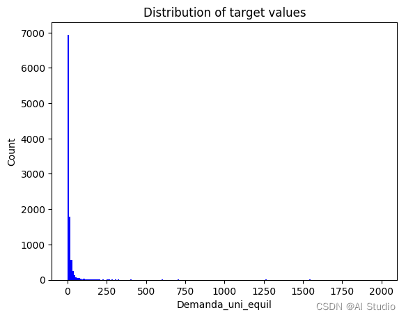
target = train['Demanda_uni_equil'].tolist()

def label_plot(title, x, y):
    plt.title(title)
    plt.xlabel(x)
    plt.ylabel(y)

plt.hist(target, bins=200, color='blue')
label_plot('Distribution of target values', 'Demanda_uni_equil', 'Count')
plt.show()

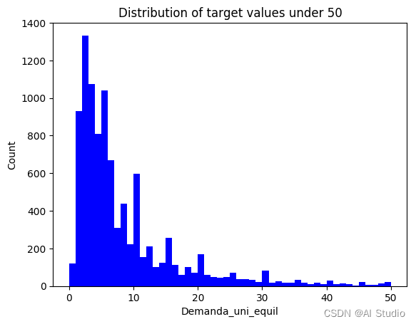
print("Looks like we have some pretty big outliers, let's zoom in and try again")

print('Data with target values under 50: ' + str(round(len(train.loc[train['Demanda_uni_equil'] <= 50]) / 5000, 2)) + '%')

plt.hist(target, bins=50, color='blue', range=(0, 50))
label_plot('Distribution of target values under 50', 'Demanda_uni_equil', 'Count')
plt.show()

Looks like we have some pretty big outliers, let's zoom in and try again
Data with target values under 50: 1.93%

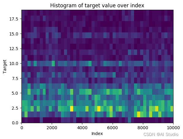
from collections import Counter
print(Counter(target).most_common(10))
print('Our most common value is 2')

[(2, 1333), (3, 1073), (5, 1041), (1, 929), (4, 809), (6, 668), (10, 598), (8, 439), (7, 309), (15, 255)]
Our most common value is 2

pseudo_time = train.loc[train.Demanda_uni_equil < 20].index.tolist()
target = train.loc[train.Demanda_uni_equil < 20].Demanda_uni_equil.tolist()

plt.hist2d(pseudo_time, target, bins=[50,20])
label_plot('Histogram of target value over index', 'Index', 'Target')
plt.show()

#去除掉多余的一列
ids = test['id']
test = test.drop(['id'],axis = 1)

print('Train subset shape: ', train.shape)
print('Train head\n',train.iloc[1:6,:])
print('\nTest head\n',test.iloc[1:6,:])

y = train['Demanda_uni_equil']
X = train[test.columns.values]

print(X.shape, y.shape)

Train subset shape:  (10000, 11)
Train head
    Semana  Agencia_ID  Canal_ID  Ruta_SAK  Cliente_ID  Producto_ID  \
1       3        1110         7      3301       15766         1216   
2       3        1110         7      3301       15766         1238   
3       3        1110         7      3301       15766         1240   
4       3        1110         7      3301       15766         1242   
5       3        1110         7      3301       15766         1250   

   Venta_uni_hoy  Venta_hoy  Dev_uni_proxima  Dev_proxima  Demanda_uni_equil  
1              4      33.52                0          0.0                  4  
2              4      39.32                0          0.0                  4  
3              4      33.52                0          0.0                  4  
4              3      22.92                0          0.0                  3  
5              5      38.20                0          0.0                  5  

Test head
    Semana  Agencia_ID  Canal_ID  Ruta_SAK  Cliente_ID  Producto_ID
1      11        2237         1      1226     4705135         1238
2      10        2045         1      2831     4549769        32940
3      11        1227         1      4448     4717855        43066
4      11        1219         1      1130      966351         1277
5      11        1146         4      6601     1741414          972
(10000, 6) (10000,)

def rmsle_func(truths, preds):
    truths = np.asarray(truths)
    preds = np.asarray(preds)
    
    n = len(truths)
    diff = (np.log(preds+1) - np.log(truths+1))**2
    print(diff, n, np.sum(diff))
    return np.sqrt(np.sum(diff)/n)

# split into train and test
X_train, X_test, y_train, y_test = train_test_split(X, y, test_size=0.2, random_state=1729)
print(X_train.shape, X_test.shape)

# logistic classifier from xgboost
rmsle  = make_scorer(rmsle_func, greater_is_better=False)

xlf = xgb.XGBRegressor(objective="reg:linear", seed=1729)
xlf.fit(X_train, y_train, eval_metric='rmse', verbose = True, eval_set = [(X_test, y_test)])

# calculate the auc score
preds = xlf.predict(X_test)

print('\nMean Square error" ', mean_squared_error(y_test,preds))

(8000, 6) (2000, 6)
[20:14:14] WARNING: ../src/objective/regression_obj.cu:170: reg:linear is now deprecated in favor of reg:squarederror.
[0]	validation_0-rmse:30.34583
[1]	validation_0-rmse:28.00715
[2]	validation_0-rmse:27.12540
[3]	validation_0-rmse:26.66389
[4]	validation_0-rmse:26.29345
[5]	validation_0-rmse:27.15917
[6]	validation_0-rmse:27.43757
[7]	validation_0-rmse:28.75123
[8]	validation_0-rmse:28.73189
[9]	validation_0-rmse:30.20388
[10]	validation_0-rmse:30.32202
[11]	validation_0-rmse:30.51755
[12]	validation_0-rmse:30.61906
[13]	validation_0-rmse:30.51401
[14]	validation_0-rmse:30.45616
[15]	validation_0-rmse:30.28859
[16]	validation_0-rmse:30.34120
[17]	validation_0-rmse:30.33650
[18]	validation_0-rmse:30.37687
[19]	validation_0-rmse:30.44277
[20]	validation_0-rmse:30.44665
[21]	validation_0-rmse:30.44889
[22]	validation_0-rmse:30.69853
[23]	validation_0-rmse:30.69749
[24]	validation_0-rmse:30.71684
[25]	validation_0-rmse:30.71721
[26]	validation_0-rmse:30.84672
[27]	validation_0-rmse:30.93807
[28]	validation_0-rmse:31.09822
[29]	validation_0-rmse:31.01057
[30]	validation_0-rmse:31.05564
[31]	validation_0-rmse:30.96434
[32]	validation_0-rmse:30.88193
[33]	validation_0-rmse:30.85133
[34]	validation_0-rmse:31.51480
[35]	validation_0-rmse:31.52124
[36]	validation_0-rmse:31.54875
[37]	validation_0-rmse:31.56342
[38]	validation_0-rmse:31.52124
[39]	validation_0-rmse:31.52483
[40]	validation_0-rmse:31.53973
[41]	validation_0-rmse:31.46044
[42]	validation_0-rmse:31.50757
[43]	validation_0-rmse:31.51247
[44]	validation_0-rmse:31.52416
[45]	validation_0-rmse:31.53694
[46]	validation_0-rmse:31.56202
[47]	validation_0-rmse:31.63332
[48]	validation_0-rmse:31.66757
[49]	validation_0-rmse:31.67119
[50]	validation_0-rmse:31.65735
[51]	validation_0-rmse:31.63961
[52]	validation_0-rmse:31.65975
[53]	validation_0-rmse:31.67637
[54]	validation_0-rmse:31.66679
[55]	validation_0-rmse:31.65528
[56]	validation_0-rmse:31.66384
[57]	validation_0-rmse:31.67088
[58]	validation_0-rmse:31.70247
[59]	validation_0-rmse:31.85863
[60]	validation_0-rmse:31.83387
[61]	validation_0-rmse:31.83894
[62]	validation_0-rmse:31.94002
[63]	validation_0-rmse:31.96835
[64]	validation_0-rmse:32.04978
[65]	validation_0-rmse:32.07721
[66]	validation_0-rmse:32.17711
[67]	validation_0-rmse:32.17323
[68]	validation_0-rmse:32.17859
[69]	validation_0-rmse:32.17110
[70]	validation_0-rmse:32.16456
[71]	validation_0-rmse:32.17088
[72]	validation_0-rmse:32.25761
[73]	validation_0-rmse:32.26345
[74]	validation_0-rmse:32.25527
[75]	validation_0-rmse:32.43781
[76]	validation_0-rmse:32.40650
[77]	validation_0-rmse:32.40338
[78]	validation_0-rmse:32.39871
[79]	validation_0-rmse:32.39678
[80]	validation_0-rmse:32.54718
[81]	validation_0-rmse:32.56033
[82]	validation_0-rmse:32.56994
[83]	validation_0-rmse:32.57530
[84]	validation_0-rmse:32.59045
[85]	validation_0-rmse:32.59536
[86]	validation_0-rmse:32.60280
[87]	validation_0-rmse:32.60166
[88]	validation_0-rmse:32.70923
[89]	validation_0-rmse:32.71774
[90]	validation_0-rmse:32.71254
[91]	validation_0-rmse:32.76879
[92]	validation_0-rmse:32.76251
[93]	validation_0-rmse:32.79826
[94]	validation_0-rmse:32.80435
[95]	validation_0-rmse:32.80440
[96]	validation_0-rmse:32.80259
[97]	validation_0-rmse:32.86562
[98]	validation_0-rmse:32.86119
[99]	validation_0-rmse:32.87680

Mean Square error"  1080.8837711699991

#对于送入网络的输入，做个归一化。
print(X.columns)
Xdata=X
for i in X.columns:
    print(i)
    Xdata[i]=X[i]/max(X[i])
print(Xdata.describe())

Index(['Semana', 'Agencia_ID', 'Canal_ID', 'Ruta_SAK', 'Cliente_ID',
       'Producto_ID'],
      dtype='object')
Semana
Agencia_ID
Canal_ID
Ruta_SAK
Cliente_ID
Producto_ID
        Semana    Agencia_ID      Canal_ID      Ruta_SAK    Cliente_ID  \
count  10000.0  10000.000000  10000.000000  10000.000000  10000.000000   
mean       1.0      0.999279      0.555936      0.818623      0.172943   
std        0.0      0.000359      0.248449      0.265541      0.170236   
min        1.0      0.999100      0.090909      0.285674      0.001629   
25%        1.0      0.999100      0.636364      0.942066      0.010966   
50%        1.0      0.999100      0.636364      0.944349      0.139843   
75%        1.0      0.999100      0.636364      0.946347      0.240926   
max        1.0      1.000000      1.000000      1.000000      1.000000   

        Producto_ID  
count  10000.000000  
mean       0.292031  
std        0.339464  
min        0.001484  
25%        0.024642  
50%        0.063922  
75%        0.644282  
max        1.000000  


/opt/conda/envs/python35-paddle120-env/lib/python3.7/site-packages/ipykernel_launcher.py:6: SettingWithCopyWarning: 
A value is trying to be set on a copy of a slice from a DataFrame.
Try using .loc[row_indexer,col_indexer] = value instead

See the caveats in the documentation: https://pandas.pydata.org/pandas-docs/stable/user_guide/indexing.html#returning-a-view-versus-a-copy

import paddle

class MyModel(paddle.nn.Layer):
    # self代表类的实例自身
    def __init__(self):
        # 初始化父类中的一些参数
        super(MyModel, self).__init__()
        self.fc1 = paddle.nn.Linear(in_features=6, out_features=1)
        #self.ru=paddle.nn.ReLU()

    def forward(self, inputs):
 

        x = self.fc1(inputs)
  
        return x

model = MyModel()

opt = paddle.optimizer.SGD(learning_rate=0.001, parameters=model.parameters())

W0313 20:16:56.765470   136 gpu_resources.cc:61] Please NOTE: device: 0, GPU Compute Capability: 7.0, Driver API Version: 11.2, Runtime API Version: 11.2
W0313 20:16:56.770395   136 gpu_resources.cc:91] device: 0, cuDNN Version: 8.2.

Xdata

	Semana	Agencia_ID	Canal_ID	Ruta_SAK	Cliente_ID	Producto_ID
0	1.0	0.9991	0.636364	0.942066	0.001629	0.024642
1	1.0	0.9991	0.636364	0.942066	0.001629	0.024723
2	1.0	0.9991	0.636364	0.942066	0.001629	0.025170
3	1.0	0.9991	0.636364	0.942066	0.001629	0.025211
4	1.0	0.9991	0.636364	0.942066	0.001629	0.025252
...	...	...	...	...	...	...
9995	1.0	1.0000	0.090909	0.286530	0.005159	0.022873
9996	1.0	1.0000	0.090909	0.286530	0.005159	0.022954
9997	1.0	1.0000	0.090909	0.286530	0.005159	0.023300
9998	1.0	1.0000	0.090909	0.286530	0.005159	0.023381
9999	1.0	1.0000	0.090909	0.286530	0.005159	0.023584

10000 rows × 6 columns

EPOCH_NUM = 5   # 设置外层循环次数
BATCH_SIZE = 2  # 设置batch大小
model.train()
# 定义外层循环
for epoch_id in range(EPOCH_NUM):
    print('epoch{}'.format(epoch_id))
    # 将训练数据进行拆分，每个batch包含10条数据
    mini_batches = [(Xdata[k:k+BATCH_SIZE],y[k:k+BATCH_SIZE]) for k in range(0, len(train), BATCH_SIZE)]
    #print(mini_batches)
    for iter_id, mini_batch in enumerate(mini_batches):
        x_data=np.array(mini_batch[0],dtype='float32')
        y_label =np.array(mini_batch[1],dtype='float32') # 获得当前批次训练标签
        # 将numpy数据转为飞桨动态图tensor的格式
        features = paddle.to_tensor(x_data)
        y_label = paddle.to_tensor(y_label)
        # 前向计算
        predicts = model(features)
        # 计算损失
        loss = paddle.nn.functional.square_error_cost(predicts, y_label)
        avg_loss = paddle.mean(loss)
        # 反向传播，计算每层参数的梯度值
        avg_loss.backward()
        # 更新参数，根据设置好的学习率迭代一步
        opt.step()
        # 清空梯度变量，以备下一轮计算
        opt.clear_grad()

epoch0
epoch1
epoch2
epoch3
epoch4

模型集成与预测结果

获取sklearn和网络输出的结果，按比例求和，预测之后地区订单的需求量

test_x1=X.iloc[1:10,:]
test_x2=Xdata.iloc[1:10,:]
oc[1:10,:]
num=len(test)

y1=xlf.predict(test_x1)
y2=model(paddle.to_tensor(test_x2.to_numpy(),dtype='float32'))
y=0.5*y1+0.5*np.array(y2[:,0])

for i in range(len(y)):
    print('月份：{} 货物ID: {} 客户ID{} 预测需求量{}'.format(train['Semana'][i],train['Producto_ID'][i],train['Canal_ID'][i],int(y[i])))
    

月份：3 货物ID: 1212 客户ID7 预测需求量3
月份：3 货物ID: 1216 客户ID7 预测需求量3
月份：3 货物ID: 1238 客户ID7 预测需求量3
月份：3 货物ID: 1240 客户ID7 预测需求量3
月份：3 货物ID: 1242 客户ID7 预测需求量3
月份：3 货物ID: 1250 客户ID7 预测需求量3
月份：3 货物ID: 1309 客户ID7 预测需求量3
月份：3 货物ID: 3894 客户ID7 预测需求量3
月份：3 货物ID: 4085 客户ID7 预测需求量3

Ref

Blog

用户购买预测比赛第十名方案——纯机器学习实现

项目总结

参加本次达人营收获很多，制作项目过程中更是丰富了实践经验。在本次项目中，回归模型是解决问题的主要方法之一，因为我们需要预测产品的销售量，这是一个连续变量的问题。为了建立一个准确的回归模型，项目采取了以下步骤：

1. 数据预处理：在训练模型之前，包括数据清洗、异常值处理等。这些步骤可以提高模型的预测准确性和稳定性。(仅仅在网络模型前使用，sklearn没有处理。)

2. 模型选择：在选择回归模型时，我比较了多种不同的算法，包括线性回归、决策树、随机森林等。最终选择了回归模型的集成。

3. 超参数调整：在训练模型之前，花费了大量时间来调整模型的超参数，以达到最佳的性能。这包括调整学习率、训练epoch、batch等。

总的来说，本次项目让我深刻认识到回归模型在解决实际问题中的重要性。通过不断的尝试和调整，项目最终可以运行，同时也积累了宝贵的经验和技能。我相信，这些经验和技能在将来的数据挖掘竞赛和实际应用中都会非常有用。
（感谢指导老师，顾老师的指导。）